

High-order finite-difference seismic forward modeling method for fluid-solid boundary coupling media
-
摘要: 本文针对流固边界耦合介质提出了一种高效、稳定的正演数值模拟方法. 首先,从一阶位移-应力弹性波方程出发,基于海底流固边界的位移和应力的连续性条件,采用三次样条海底界面定量表征方法,推导出不规则海底界面下流固边界耦合介质中的地震波波动方程;其次,通过空间微分的高阶差分格式提高数值模拟的空间精度,并结合已推导的地震波波动方程,将四阶时间微分转换至高阶空间微分,进一步提高了数值模拟的时间精度;最后,在与标量波波动方程数值模拟结果对比分析的基础上,分别利用简单的水平层状模型和复杂海底模型,验证和讨论了本文提出的流固边界耦合介质高阶有限差分地震波正演模拟方法的有效性和准确性.Abstract: This paper proposes a novel and stable forward modeling method, which can describe the wave propagation through fluid-solid coupled media. Firstly, we deduce the seismic wave equations of fluid-solid coupled media with irregular interface of seabed utilizing the cubic-spline quantitative method based on the continuity of stress and displacement of the interface. And then, the high-order differential scheme for spatial differentiation is introduced into the method above, which can improve the spatial accuracy of numerical simulation. Furthermore, we also suppress the time discretization that reduces the numerical dispersion by transforming the fourth-order time differential into higher-order spatial differential method. Finally, comparing with results of the scalar wave equation and numerical simulation, we analyze the numerical results of the method proposed in this paper for a simple horizontal layered model and a complex one. The numerical simulation of wave propagation in the fluid-solid coupled media indicates that the method proposed in this paper is convenient and accurate.
-
Keywords:
- seismic forward /
- finite difference /
- scalar wave /
- elastic wave /
- fluid-solid boundary
-
引言
海洋地震勘探中地震波在流固边界相互耦合的介质中传播时,通常采用拖缆地震采集或海底地震采集两种方式来获取数据,两种方式的地震激发均在水中完成. 流体介质的本质特征是横波模量为零,因此深水地震勘探中地震波传播介质可以抽象为上覆液相弹性介质或上覆零横波模量弹性介质,深水地震勘探应获取与横波模量相关的纵波或转换纵波数据. 地震波在海水中传播时,用标量波波动方程描述;当地震波穿过海底进入固相介质后,则由弹性波波动方程描述(Lee et al,2009 ;Cho et al,2016 ). 如果只用声波理论模拟整个过程,波形反演得到的结果则不可信(Choi et al,2008 ),本文的目的即是针对流固边界耦合介质建立波动方程.
波动方程的数值模拟方法有有限差分法、有限元法和伪谱法等. 由于海底界面不规则,Zhang (2004)通过有限元法正演模拟来适应海底起伏的地表;Lee等(2009)在Zhang (2004)的基础上采用规则剖分网格的建模算法,可将算法应用于全波形反演和逆时偏移,并使用Reynolds (1978)和Higdon (1991)提出的吸收边界,但该算法差分精度过低;Virieux (1986)和Levander (1988)提出交错网格有限差分算法模拟弹性波一阶应力-速度方程的数值解,在此基础上Yu等(2016)通过将声波方程带入弹性波方程实现了流固边界耦合介质的逆时偏移.
This page contains the following errors:
error on line 1 at column 1: Start tag expected, '<' not foundBelow is a rendering of the page up to the first error.
鉴于此,本文首先推导不规则流固边界耦合介质下的地震波波动方程,正演采用规则网格剖分,用三次样条函数表征海底界面起伏;其次,基于完美匹配层(perfect matched layer,简写为PML)边界将时间差分精度由二阶推广至四阶,在不增加计算机内存和不降低计算效率前提下压制时间频散;最后,分别采用上覆流体的水平层状模型和凹陷模型进行测试,以验证本文算法的有效性和可行性.
1. 流固边界耦合介质波动方程
1.1 流体介质标量波方程
在海洋地震勘探中,因为在海水液相介质中剪切模量为零,如果均采用弹性波方程来求解,则在剪切模量为零区域会导致奇异性,致使求解过程不稳定;若仅使用标量波方程求解,则得不到海底弹性介质中的转换波,因此地震波在耦合介质中传播需分为两部分来描述:液相介质中传播可以通过标量波波动方程来描述;固相介质中的传播用弹性波方程来描述. 因此构建该环境下的波动方程,需要分析流相和固相介质中波的传播规律.
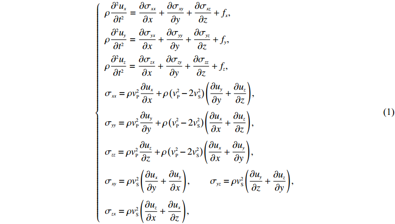
在流固边界耦合介质中,标量波动方程其实是从弹性波方程推导而来. 相比于固相介质,流体中横波速度为零,因此分析标量波动方程,可以先从弹性介质波动方程入手:
$ \left\{ \begin{array}{l}\rho \displaystyle\frac{{{\partial ^2}{u_x}}}{{\partial {t^2}}} = \frac{{\partial {\sigma _{xx}}}}{{\partial x}} + \frac{{\partial {\sigma _{xy}}}}{{\partial y}} + \frac{{\partial {\sigma _{xz}}}}{{\partial z}} + {f_x},\\[10pt]\rho \displaystyle\frac{{{\partial ^2}{u_y}}}{{\partial {t^2}}} = \frac{{\partial {\sigma _{yx}}}}{{\partial x}} + \frac{{\partial {\sigma _{yy}}}}{{\partial y}} + \frac{{\partial {\sigma _{yz}}}}{{\partial z}} + {f_y},\\[10pt]\rho \displaystyle\frac{{{\partial ^2}{u_z}}}{{\partial {t^2}}} = \frac{{\partial {\sigma _{zx}}}}{{\partial x}} + \frac{{\partial {\sigma _{zy}}}}{{\partial y}} + \frac{{\partial {\sigma _{zz}}}}{{\partial z}} + {f_z},\\[10pt]{\sigma _{xx}} = \rho v_{{P}}^2 \displaystyle\frac{{\partial {u_x}}}{{\partial x}} + \rho \left( {v_{{P}}^2 - {{2}}v_{{S}}^2} \right)\left( {\frac{{\partial {u_y}}}{{\partial y}} + \frac{{\partial {u_z}}}{{\partial z}}} \right),\\[12pt]{\sigma _{yy}} = \rho v_{{P}}^2 \displaystyle\frac{{\partial {u_y}}}{{\partial y}} + \rho \left( {v_{{P}}^2 - {{2}}v_{{S}}^2} \right)\left( {\frac{{\partial {u_x}}}{{\partial x}} + \displaystyle\frac{{\partial {u_z}}}{{\partial z}}} \right),\\[12pt]{\sigma _{zz}} = \rho v_{{P}}^2\displaystyle\frac{{\partial {u_z}}}{{\partial z}} + \rho \left( {v_{{P}}^2 - {{2}}v_{{S}}^2} \right)\left( {\displaystyle\frac{{\partial {u_x}}}{{\partial x}} + \displaystyle\frac{{\partial {u_y}}}{{\partial y}}} \right),\\[12pt]{\sigma _{xy}} = \rho v_{{S}}^2\left( {\displaystyle\frac{{\partial {u_x}}}{{\partial y}} + \frac{{\partial {u_y}}}{{\partial x}}} \right),\quad\quad {\sigma _{yz}} = \rho v_{{S}}^2\left( {\displaystyle\frac{{\partial {u_y}}}{{\partial z}} + \frac{{\partial {u_z}}}{{\partial y}}} \right),\\[13pt]{\sigma _{zx}} = \rho v_{{S}}^2\left( {\displaystyle\frac{{\partial {u_z}}}{{\partial x}} + \frac{{\partial {u_x}}}{{\partial z}}} \right),\end{array} \right.$
(1) This page contains the following errors:
error on line 1 at column 1: Start tag expected, '<' not foundBelow is a rendering of the page up to the first error.
$\setcounter{equation}{2}{{{C}}_{{f}}}{{ = }}\left({\begin{array}{*{20}{c}}{\rho v_{{P}}^2}&{\rho v_{{P}}^2}&{\rho v_{{P}}^2}&0&0&0\\[1pt]{\rho v_{{P}}^2}&{\rho v_{{P}}^2}&{\rho v_{{P}}^2}&0&0&0\\[1pt]{\rho v_{{P}}^2}&{\rho v_{{P}}^2}&{\rho v_{{P}}^2}&0&0&0\\[1pt]0&0&0&{{0}}&0&0\\[1pt]0&0&0&0&{{0}}&0\\[1pt]0&0&0&0&0&{{0}}\end{array}} \right), $
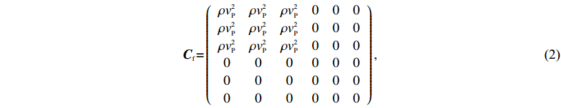
(2) 通过式(2)可以建立地震波在流体中传播的矢量方程
$\rho \frac{{{\partial ^2}{{u}}}}{{\partial {t^2}}}{{ = }}\rho v_{{P}}^2\nabla \left({\nabla { \bullet } {{u}}} \right){{ + }}{{F}}, $

(3) This page contains the following errors:
error on line 1 at column 1: Start tag expected, '<' not foundBelow is a rendering of the page up to the first error.
$\rho \frac{{{\partial ^2}{{u}}}}{{\partial {t^2}}}{{ = }} - \nabla p{{ + }}{{F}}, $

(4) 对式(4)等号两边求散度得到流体介质中描述纵波传播的标量波方程
$\left({\frac{{{\partial ^{{2}}}}}{{\partial {t^{{2}}}}} - {{{C}}_{{f}}}{{{L}}_{{f}}}} \right)p = f, $

(5) This page contains the following errors:
error on line 1 at column 1: Start tag expected, '<' not foundBelow is a rendering of the page up to the first error.
1.2 固体介质弹性波方程
基于式(1)给出的弹性波位移-应力方程,利用本构方程和几何方程建立三维弹性波纯位移方程如下:
$\left({\rho \frac{{{\partial ^{{2}}}}}{{\partial {t^{{2}}}}} - {{{L}}_{{s}}}{{{C}}_{{s}}}{{L}}_{{s}}^{{T}}} \right){{u}} = {{F}}, $

(6) This page contains the following errors:
error on line 1 at column 1: Start tag expected, '<' not foundBelow is a rendering of the page up to the first error.
${{{L}}_{{s}}}{{ = }}\left({\begin{array}{*{20}{c}}{{\partial _x}}&0&0&0&{{\partial _z}}&{{\partial _y}}\\[1pt]0&{{\partial _y}}&0&{{\partial _z}}&0&{{\partial _x}}\\[1pt]0&0&{{\partial _z}}&{{\partial _y}}&{{\partial _x}}&0\end{array}} \right); $

(7) This page contains the following errors:
error on line 7 at column 23: Extra content at the end of the documentBelow is a rendering of the page up to the first error.
${{{C}}_{{s}}}$
${{{C}}_{{s}}}{{ = }}\left({\begin{array}{*{20}{c}}{\rho v_{{P}}^2}&{\rho v_{{P}}^2 - 2\rho v_{{S}}^2}&{\rho v_{{P}}^2 - 2\rho v_{{S}}^2}&0&0&0\\[3pt]{\rho v_{{P}}^2 - 2\rho v_{{S}}^2}&{\rho v_{{P}}^2}&{\rho v_{{P}}^2 - 2\rho v_{{S}}^2}&0&0&0\\[3pt]{\rho v_{{P}}^2 - 2\rho v_{{S}}^2}&{\rho v_{{P}}^2 - 2\rho v_{{S}}^2}&{\rho v_{{P}}^2}&0&0&0\\[3pt]0&0&0&{\rho v_{{S}}^2}&0&0\\[3pt]0&0&0&0&{\rho v_{{S}}^2}&0\\[3pt]0&0&0&0&0&{\rho v_{{S}}^2}\end{array}} \right){\text{.}} $
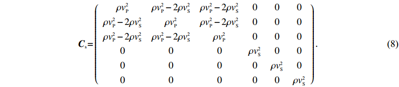
(8) 海上勘探震源激发在水中完成,而海底介质是无源的,即F=0,则可用
$\left\{\!\!\! \begin{array}{l}\displaystyle\frac{{{\partial ^{{2}}}{u_x}}}{{\partial {t^2}}} = v_{{P}}^2\left({\frac{{{\partial ^2}{u_x}}}{{\partial {x^2}}} + \frac{{{\partial ^2}{u_y}}}{{\partial x\partial y}} + \frac{{{\partial ^2}{u_z}}}{{\partial x\partial z}}} \right) + v_{{S}}^2\left({\frac{{{\partial ^2}{u_x}}}{{\partial {y^2}}} + \frac{{{\partial ^2}{u_x}}}{{\partial {z^2}}} - \frac{{{\partial ^{{2}}}{u_y}}}{{\partial x\partial y}} - \frac{{{\partial ^{{2}}}{u_z}}}{{\partial x\partial z}}} \right), \\[13pt]\displaystyle\frac{{{\partial ^{{2}}}{u_y}}}{{\partial {t^2}}} = v_{{P}}^2\left({\frac{{{\partial ^2}{u_x}}}{{\partial x\partial y}} + \frac{{{\partial ^2}{u_y}}}{{\partial {y^2}}} + \frac{{{\partial ^2}{u_z}}}{{\partial y\partial z}}} \right) + v_{{S}}^2\left({\frac{{{\partial ^2}{u_y}}}{{\partial {x^2}}} + \frac{{{\partial ^2}{u_y}}}{{\partial {z^2}}} - \frac{{{\partial ^{{2}}}{u_x}}}{{\partial x\partial y}} - \frac{{{\partial ^{{2}}}{u_z}}}{{\partial y\partial z}}} \right), \\[13pt]\displaystyle\frac{{{\partial ^{{2}}}{u_z}}}{{\partial {t^2}}} = v_{{P}}^2\left({\frac{{{\partial ^2}{u_x}}}{{\partial x\partial z}} + \frac{{{\partial ^2}{u_y}}}{{\partial y\partial z}} + \frac{{{\partial ^2}{u_z}}}{{\partial {z^2}}}} \right) + v_{{S}}^2\left({\frac{{{\partial ^2}{u_z}}}{{\partial {x^2}}} + \frac{{{\partial ^2}{u_z}}}{{\partial {y^2}}} - \frac{{{\partial ^{{2}}}{u_x}}}{{\partial x\partial z}} - \frac{{{\partial ^{{2}}}{u_y}}}{{\partial y\partial z}}} \right)\end{array} \right.$
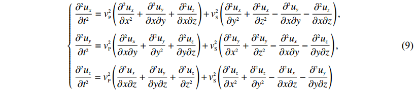
(9) 描述地震波在海底固相介质中的传播.
1.3 流固边界耦合介质边界条件
本文利用正应力方向的位移和应力连续条件建立地震波在流固耦合介质分界面的转换方程. 水中地震波传播至海底,对海底面(流固分界面)产生压力,而对海底的施压其实就是固相介质中弹性波传播时边界上施加牵引力. 根据应力张量定理可知,在边界上任意一点的牵引力都可用该点的应力张量来表示,牵引力与施加于海底界面上的声压是作用与反作用的关系,两者单位一致,在流固相分界面上的边界条件用应力连续这个条件进行衔接.
This page contains the following errors:
error on line 1 at column 1: Start tag expected, '<' not foundBelow is a rendering of the page up to the first error.
${{\sigma }} = {{T }} \bullet {{n}}, $

(10) This page contains the following errors:
error on line 1 at column 1: Start tag expected, '<' not foundBelow is a rendering of the page up to the first error.
$\left\{\!\!\! \begin{array}{l}{\sigma _{{n_x}}} = {n_x}{\sigma _{xx}} + {n_y}{\sigma _{yx}} + {n_z}{\sigma _{zx}}, \\[3pt]{\sigma _{{n_y}}} = {n_x}{\sigma _{xy}} + {n_y}{\sigma _{yy}} + {n_z}{\sigma _{zy}}, \\[3pt]{\sigma _{{n_z}}} = {n_x}{\sigma _{xz}} + {n_y}{\sigma _{yz}} + {n_z}{\sigma _{zz}}{\text{.}}\end{array} \right.$

(11) This page contains the following errors:
error on line 1 at column 1: Start tag expected, '<' not foundBelow is a rendering of the page up to the first error.
$\left\{\!\!\! \begin{array}{l} - p {n_x} = {n_x}{\sigma _{xx}} + {n_y}{\sigma _{xy}} + {n_z}{\sigma _{xz}}, \\[3pt] - p {n_y} = {n_x}{\sigma _{yx}} + {n_y}{\sigma _{yy}} + {n_z}{\sigma _{yz}}, \\[3pt] - p{n_z} = {n_x}{\sigma _{zx}} + {n_y}{\sigma _{zy}} + {n_z}{\sigma _{zz}}, \end{array} \right.$
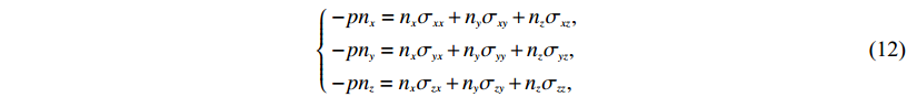
(12) 式中p为标量场. 对式(12)进行角度归一化得到耦合界面法线方向上的流体压力为
$ - p = n_x^2{\sigma _{xx}} + n_y^2{\sigma _{yy}} + n_z^2{\sigma _{zz}} + 2{n_x}{n_y}{\sigma _{xy}} + 2{n_y}{n_z}{\sigma _{zy}} + 2{n_x}{n_z}{\sigma _{xz}}{\text{.}} $

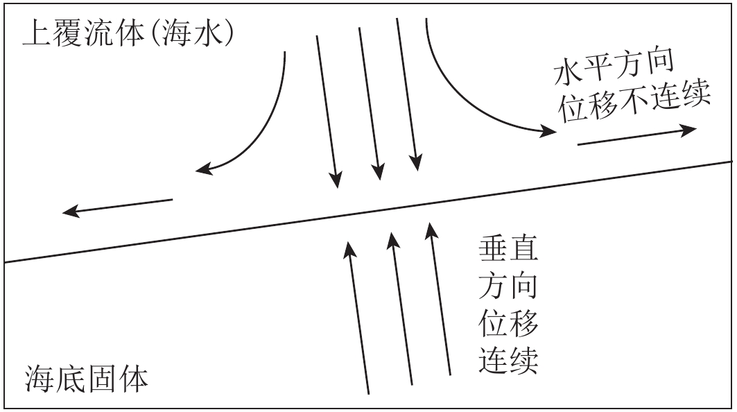
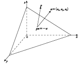
(13) 当弹性波回传到流固分界面时,根据式(13)将弹性波波场(矢量场)转换为标量场,再由本构方程和胡克定律得到位移表示下的应力连续条件. 继而在流固边界耦合介质的分界面上建立位移连续条件,考虑到质点运动位移在垂直界面方向连续,如图2所示,法向位移满足叠加原理.
![]() 图 1 流固耦合界面正应力连续
图 1 流固耦合界面正应力连续${n_x}, \ {n_y}, \ {n_z}$ 表示n与3个坐标轴夹角的余弦Figure 1. Fluid-solid coupling normal stress continuous in interface${n_x}, \ {n_y}, \ {n_z}$ represents the cosine of the angle between the n and axis![]() 图 2 流固耦合分界面法向位移连续Figure 2. Displacement continuous in normal direction at the fluid-solid coupling interface
图 2 流固耦合分界面法向位移连续Figure 2. Displacement continuous in normal direction at the fluid-solid coupling interface标量波方程不含位移项,这里需要利用位移连续条件将流体的位移转变为压力以满足波动方程
${{{u}}_{{s}}} - {{{u}}_{{f}}} = \iint\nolimits_t {\frac{{{\partial ^{{2}}}{{{u}}_{{s}}}}}{{\partial {t^{{2}}}}}} - \iint\nolimits_t {\frac{{{\partial ^{{2}}}{{{u}}_{{f}}}}}{{\partial {t^{{2}}}}}} {{ = 0}} \Rightarrow \frac{{{\partial ^{{2}}}{{{u}}_{{s}}}}}{{\partial {t^{{2}}}}} - v_{{P}}^2\nabla \left({\nabla { \bullet } {{{u}}_{{f}}}} \right){{ = }}0, $

(14) 由压缩模量和声压关系可得
$\frac{{{\partial ^{{2}}}{{{u}}_{{s}}}}}{{\partial {t^{{2}}}}} = - \frac{{{1}}}{\rho }\nabla p, $

(15) 式(15)揭示了耦合边界处位移连续条件隐含于流体压力之中,由此对式(11)求梯度可得
$\left\{\!\!\! \begin{array}{l} - \displaystyle\frac{{{1}}}{\rho }\frac{{\partial p}}{{\partial x}}{n_x} = {n_x}\frac{{{1}}}{\rho }\frac{{\partial {\sigma _{xx}}}}{{\partial x}} + {n_y}\frac{{{1}}}{\rho }\frac{{\partial {\sigma _{xy}}}}{{\partial x}} + {n_z}\frac{{{1}}}{\rho }\frac{{\partial {\sigma _{xz}}}}{{\partial x}}, \\[11pt] - \displaystyle\frac{{{1}}}{\rho }\frac{{\partial p}}{{\partial y}}{n_y} = {n_x}\frac{{{1}}}{\rho }\frac{{\partial {\sigma _{yx}}}}{{\partial y}} + {n_y}\frac{{{1}}}{\rho }\frac{{\partial {\sigma _{yy}}}}{{\partial y}} + {n_z}\frac{{{1}}}{\rho }\frac{{\partial {\sigma _{yz}}}}{{\partial y}}, \\[11pt] - \displaystyle\frac{{{1}}}{\rho }\frac{{\partial p}}{{\partial z}}{n_z} = {n_x}\frac{{{1}}}{\rho }\frac{{\partial {\sigma _{zx}}}}{{\partial z}} + {n_y}\frac{{{1}}}{\rho }\frac{{\partial {\sigma _{zy}}}}{{\partial z}} + {n_z}\frac{{{1}}}{\rho }\frac{{\partial {\sigma _{zz}}}}{{\partial z}}, \end{array} \right.$
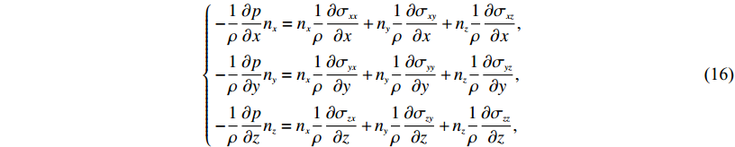
(16) 将式(16)合并得到
$\begin{split} & - \displaystyle\frac{{{1}}}{\rho }\left({\frac{{\partial p}}{{\partial x}}{n_x} + \frac{{\partial p}}{{\partial y}}{n_y} + \frac{{\partial p}}{{\partial z}}{n_z}} \right) = \frac{{{1}}}{\rho }\left({\frac{{\partial {\sigma _{xx}}}}{{\partial x}} + \frac{{\partial {\sigma _{yx}}}}{{\partial y}} + \frac{{\partial {\sigma _{zx}}}}{{\partial z}}} \right){n_x} + \displaystyle\frac{{{1}}}{\rho }\left({\frac{{\partial {\sigma _{xy}}}}{{\partial x}} + \frac{{\partial {\sigma _{yy}}}}{{\partial y}} + \frac{{\partial {\sigma _{zy}}}}{{\partial z}}} \right){n_y}+\\[3pt] & \qquad\qquad\qquad\qquad\qquad\qquad\quad \displaystyle\frac{{{1}}}{\rho }\left({\frac{{\partial {\sigma _{xz}}}}{{\partial x}} + \frac{{\partial {\sigma _{yz}}}}{{\partial y}} + \frac{{\partial {\sigma _{zz}}}}{{\partial z}}} \right){n_z}, \end{split}$
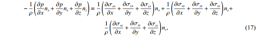
(17) 式(17)右端项即为弹性介质的3个分量,由此得到耦合边界上位移连续条件,利用该条件即可将液相介质中的标量场转换为固相中的矢量场
$\left({\frac{{{\partial ^2}{u_x}}}{{\partial {t^2}}}{{ + }}\frac{1}{\rho }\frac{{\partial p}}{{\partial x}}} \right){n_x} + \left({\frac{{{\partial ^2}{u_y}}}{{\partial {t^2}}}{{ + }}\frac{1}{\rho }\frac{{\partial p}}{{\partial y}}} \right){n_y} + \left({\frac{{{\partial ^2}{u_z}}}{{\partial {t^2}}}{{ + }}\frac{1}{\rho }\frac{{\partial p}}{{\partial z}}} \right){n_z} = 0. $

(18) 1.4 流固边界耦合介质波动方程
根据上述条件建立流固边界耦合介质波动方程
$\left({\frac{{{\partial ^2}}}{{\partial {t^2}}} - {{ D}}{{ N}}{{{ C}}_{{c}}}{{{ L}}_{{c}}}} \right){{\varPhi}} + {{F}} = 0, $

(19) This page contains the following errors:
error on line 1 at column 1: Start tag expected, '<' not foundBelow is a rendering of the page up to the first error.
${{{C}}_{{c}}} = \left({\begin{array}{*{20}{c}}{v_{{P}}^2}&{{0}}&{{0}}&{{0}}&{{0}}&{{0}}&{{0}}\\[1pt]{{0}}&{v_{{P}}^2}&{v_{{P}}^2 - {{2}}v_{{S}}^2}&{v_{{P}}^2 - {{2}}v_{{S}}^2}&{{0}}&{{0}}&{{0}}\\[1pt]{{0}}&{v_{{P}}^2 - {{2}}v_{{S}}^2}&{v_{{P}}^2}&{v_{{P}}^2 - {{2}}v_{{S}}^2}&{{0}}&{{0}}&{{0}}\\[1pt]{{0}}&{v_{{P}}^2 - {{2}}v_{{S}}^2}&{v_{{P}}^2 - {{2}}v_{{S}}^2}&{v_{{P}}^2}&{{0}}&{{0}}&{{0}}\\[1pt]{{0}}&{{0}}&{{0}}&{{0}}&{v_{{S}}^2}&{{0}}&{{0}}\\[1pt]{{0}}&{{0}}&{{0}}&{{0}}&{{0}}&{v_{{S}}^2}&{{0}}\\[1pt]{{0}}&{{0}}&{{0}}&{{0}}&{{0}}&{{0}}&{v_{{S}}^2}\end{array}} \right); $
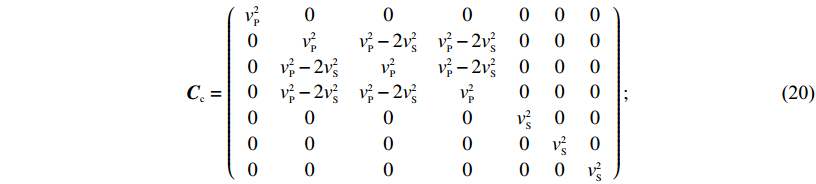
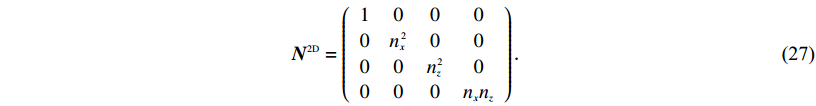
(20) N为耦合界面方向矩阵,界面之外介质方向因子值取单位1,
${{N}} = \left({\begin{array}{*{20}{c}}1&0&0&0&0&0&0\\[1pt]0&{{n_x}\!\!^2}&0&0&0&0&0\\[1pt]0&0&{{n_y}\!\!^2}&0&0&0&0\\[1pt]0&0&0&{{n_z}\!\!^2}&0&0&0\\[1pt]0&0&0&0&{{n_y}{n_z}}&0&0\\[1pt]0&0&0&0&0&{{n_z}{n_x}}&0\\[1pt]0&0&0&0&0&0&{{n_x}{n_y}}\end{array}} \right); $
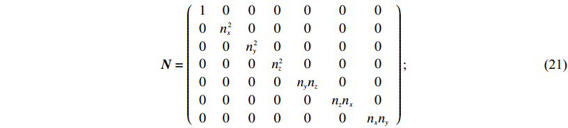
(21) This page contains the following errors:
error on line 7 at column 23: Extra content at the end of the documentBelow is a rendering of the page up to the first error.
${{{L}}_{{c}}}$
${{{L}}_{{c}}}{{ = }}{\left({\begin{array}{*{20}{c}}{{1}}&{{0}}&{{0}}&{{0}}&{{0}}&{{0}}&{{0}}\\[1pt]{{0}}&{{\partial _x}}&{{0}}&{{0}}&{{0}}&{{\partial _z}}&{{\partial _y}}\\[1pt]{{0}}&{{0}}&{{\partial _y}}&{{0}}&{{\partial _z}}&{{0}}&{{\partial _x}}\\[1pt]{{0}}&{{0}}&{{0}}&{{\partial _z}}&{{\partial _y}}&{{\partial _x}}&{{0}}\end{array}} \right)^{{T}}}, $
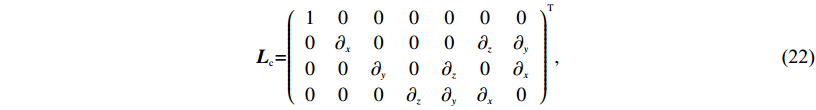
(22) ${{D}} = \left({\begin{array}{*{20}{c}}{{\nabla ^{2}}}&{{\partial _{{t^{\scriptsize 2}}}}\!\!\!\!^*}&{{\partial _{{t^2}}}\!\!\!\! ^*}&{{\partial _{{t^2}}}\!\!\!\!^*}&2{{\partial _{{t^2}}}\!\!\!\!^*}&2{{\partial _{{t^2}}}\!\!\!\!^*}&2{{\partial _{{t^2}}}\!\!\!\!^*}\\[1pt]{{\partial _x}\!\! ^*}&{{\partial _x}}&0&0&0&{{\partial _z}}&{{\partial _y}}\\[1pt]{{\partial _y}\!\!^*}&0&{{\partial _y}}&0&{{\partial _z}}&0&{{\partial _x}}\\[1pt]{{\partial _z}\!\!^*}&0&0&{{\partial _z}}&{{\partial _y}}&{{\partial _x}}&0\end{array}} \right), $
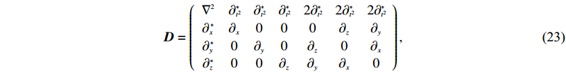
(23) 当波传播至流固耦合分界面时,*对应的元素在耦合边界以外取值为0.
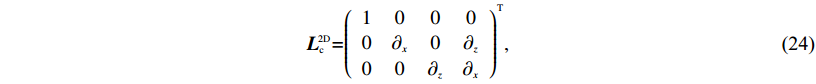
在二维各向同性介质条件下,上述矩阵表示为
${{{L}}_{{c}}}\!\!\!^{{{2D}}}{{ = }}{\left({\begin{array}{*{20}{c}}{{1}}&{{0}}&{{0}}&{{0}}\\[1pt]{{0}}&{{\partial _x}}&0&{{\partial _z}}\\[1pt]{{0}}&{{0}}&{{\partial _z}}&{{\partial _x}}\end{array}} \right)^{{T}}}, $
(24) ${{{C}}_{{c}}}\!\! ^{{{2D}}} = \left({\begin{array}{*{20}{c}}{v_{{P}}^2}&0&0&0\\[1pt]{{0}}&{v_{{P}}^2}&{v_{{P}}^2 - {{2}}v_{{S}}^2}&0\\[1pt]{{0}}&{v_{{P}}^2 - {{2}}v_{{S}}^2}&{v_{{P}}^2}&0\\[1pt]{{0}}&0&0&{v_{{S}}^2}\end{array}} \right), $
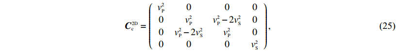
(25) ${{{D}}^{{{2D}}}} = \left({\begin{array}{*{20}{c}}{{\nabla ^2}}&{{\partial _{{t^2}}}\!\!\!^*}&{{\partial _{{t^2}}}\!\!\!\!^*}&2{{\partial _{{t^2}}}\!\!\!\!^*}\\[1pt]{{\partial _x}\!\!\!\!^*}&{{\partial _x}}&0&{{\partial _z}}\\[1pt]{{\partial _z}\!\!^*}&0&{{\partial _z}}&{{\partial _x}}\end{array}} \right), $

(26) ${{{N}}^{{{2D}}}} = \left({\begin{array}{*{20}{c}}{{1}}&0&0&0\\[1pt]0&{{n_x}\!\!^2}&0&0\\[1pt]0&0&{{n_z}\!\!^2}&0\\[1pt]0&0&0&{{n_x}{n_z}}\end{array}} \right){\text{.}}$
(27) 由此建立了流固边界耦合介质下地震波传播方程,但是现实中海水是分层,海底固相介质自上而下从淤泥过渡到成岩的介质,这些情况本文并未考虑,对于更真实、精确地描述海洋中波的传播规律,还有很多问题亟待解决.
2. 时空高阶有限差分数算法
与陆上勘探相同,提高海洋勘探的时空精度也是一个非常重要的问题. 有限差分法的固有缺陷就是数值频散.数值频散主要分为时间频散和空间频散两个方面,而时间网格和空间网格或震源主频选取不当均会产生数值频散(吴国忱,王华忠,2005),因此建立时空高阶有限差分数算法对于实际应用具有重要意义(Madariaga,1976).
以标量波波动方程为例,空间高阶有限差分格式如下:
$\left\{\!\!\! {\begin{array}{*{20}{l}}{\displaystyle\frac{{\partial p}}{{\partial x}} = \frac{1}{{\Delta x}}\sum\limits_{n = 1}^N {{c_n}\left[ {p\left( {x + n\Delta x} \right) - p\left( {x - n\Delta x} \right)} \right]} + o\left( {\Delta {x^{2N}}} \right),}\\[9pt]{\displaystyle\frac{{{\partial ^2}p}}{{\partial {x^2}}} = \frac{1}{{2\Delta {x^2}}}\left\{ {{\omega _0}p\left( x \right) + \sum\limits_{n = 1}^N {{\omega _n}\left[ {p\left( {x + n\Delta x} \right) + p\left( {x - n\Delta x} \right)} \right]} } \right\} + o\left( {\Delta {x^{2N}}} \right),}\\[9pt]{\displaystyle\frac{{{\partial ^2}p}}{{\partial x\partial z}} = \frac{1}{{\Delta x\Delta z}}\sum\limits_{\scriptstyle{n_1} = - N\hfill\atop\ \scriptstyle{n_1} \ne 0\hfill}^N {{c_{{n_1}}}} \sum\limits_{\scriptstyle{n_2} = - N\hfill\atop\ \scriptstyle{n_2} \ne 0\hfill}^N {{c_{{n_2}}}} p\left( {x + {n_1}\Delta x,z + {n_2}\Delta z} \right) + o\left( {\Delta {x^{2N}} + \Delta {z^{2N}}} \right),}\end{array}} \right.$
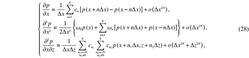
(28) This page contains the following errors:
error on line 1 at column 1: Start tag expected, '<' not foundBelow is a rendering of the page up to the first error.
通常,差分方程涉及时间层越多,对计算机的内存要求越高. 为不增加内存,本文推导了基于PML边界(Berenger,1994)下的时间四阶精度有限差分算法,以标量波波动方程为例,给出标量波时间域的PML控制方程(何燕,2008)
$\left\{\!\!\! \begin{array}{l}p = {p_x} + {p_y} + {p_z}, \\[6pt]\displaystyle\frac{{{\partial ^2}{p_i}}}{{\partial {t^2}}} + 2{d_i}\frac{{\partial {p_i}}}{{\partial t}}{\delta _{ij}} + {d_i}^2{p_j}{\delta _{ij}} = {v_{{P}}\!\!^2}\frac{{{\partial ^2}p}}{{\partial {i^2}}},\quad i,\ j=x ,\ y ,\ z {\text{.}}\end{array} \right.$

(29) 有限差分法即是对p进行泰勒级数展开从而得到相应的偏导数值(Dablain,1986),由此可以得出时间二阶导数的高阶差商和时间一阶导数差商的表达式为
$\left\{\!\!\! \begin{array}{l}\displaystyle\frac{{{\partial ^2}p\left(t \right)}}{{\partial {t^2}}} = \frac{{{1}}}{{\Delta {t^2}}}\left\{ {\left[ {p\left({t + \Delta t} \right) - 2p\left(t \right) + p\left({t - \Delta t} \right)} \right] - \frac{2}{{4!}}\frac{{{\partial ^4}p\left(t \right)}}{{\partial {t^4}}}\Delta {t^4} + \cdots } \right\}, \\[13pt]\displaystyle\frac{{\partial p\left(t \right)}}{{\partial t}} = \frac{{p\left({t + \Delta t} \right) - p\left({t - \Delta t} \right)}}{{\Delta t}}. \end{array} \right.$
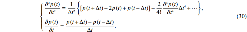
(30) 对于时间导数泰勒级数展开中的四阶导数,采取转换到空间的方式处理,以波场分裂后的x向为例,
$\frac{{{\partial ^{{4}}}{p_x}}}{{\partial {t^{{4}}}}}{{ = }}\frac{{{\partial ^2}}}{{\partial {t^2}}}\left({\frac{{{\partial ^2}{p_x}}}{{\partial {t^2}}}} \right) = \frac{{{\partial ^2}}}{{\partial {t^2}}}\left[ {v_{{P}}^2\frac{{{\partial ^2}p}}{{\partial {x^2}}} - 2{d_x}\left(x \right)\frac{{\partial {p_x}}}{{\partial t}} - {d_x}\!\!^2\left(x \right){p_x}} \right], $

(31) This page contains the following errors:
error on line 1 at column 1: Start tag expected, '<' not foundBelow is a rendering of the page up to the first error.
$\alpha {p_x}\!\!^{n + 1} - \beta {p_x}\!\!^n + \gamma {p_x}\!\!^{n - 1} = {v_{{P}}^2}\Delta {t^{{2}}}\frac{{{\partial ^2}p}}{{{\partial ^2}x}} + {M_x}, $

(32) This page contains the following errors:
error on line 1 at column 1: Start tag expected, '<' not foundBelow is a rendering of the page up to the first error.
$\left\{ \begin{align} & \alpha = {{1 + }}{d_x}\left(x \right)\Delta t{{ + }}\frac{{{1}}}{{{6}}}{d_x}\!^{{3}}\left(x \right)\Delta {t^{{3}}}, \\& \beta = 2 - {d_x}\!^2\left(x \right)\Delta {t^{{2}}} - \frac{{{1}}}{4}{d_x}\!^4\left(x \right)\Delta {t^4}, \\ & \gamma = {{1}} - {d_x}\left(x \right)\Delta t - \frac{{{1}}}{{{6}}}{d_x}\!^3\left(x \right)\Delta {t^{{3}}}, \\ & {M_x} = \displaystyle\frac{{{1}}}{{{{12}}}}v_{{P}}^4\Delta {t^4}\left({\frac{{{\partial ^2}p}}{{\partial {x^4}}}{{ + }}\frac{{{\partial ^2}p}}{{\partial {x^2}\partial {y^2}}}{{ + }}\frac{{{\partial ^2}p}}{{\partial {x^2}\partial {z^2}}}} \right) {{ + }}\displaystyle\frac{{{1}}}{4}{d_x}\!^2\left(x \right)v_{{P}}^2\Delta {t^4}\frac{{{\partial ^2}p}}{{\partial {x^2}}} - \frac{{{1}}}{{{6}}}{d_x}\left(x \right)v_{{P}}^2\Delta {t^4}\frac{{{\partial ^2}Q}}{{\partial {x^2}}}, \end{align} \right.$
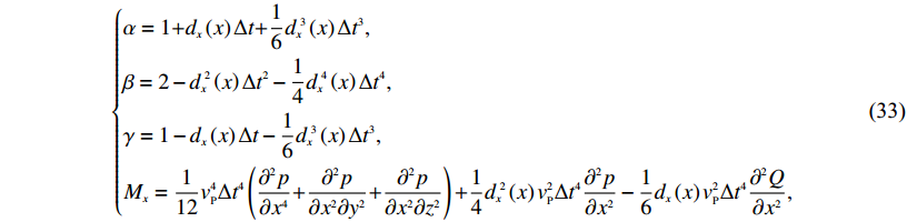
(33) 式中Q表示空间转换部分的一项积分项,
$Q = \frac{{\partial p}}{{\partial t}} = \int_{{t_0}}^t {\frac{{{\partial ^2}p}}{{\partial {t^2}}}dt} = \int_{{t_0}}^t {v_{{P}}^2\left({\frac{{{\partial ^2}p}}{{\partial {x^2}}}{{ + }}\frac{{{\partial ^2}p}}{{\partial {y^2}}}{{ + }}\frac{{{\partial ^2}p}}{{\partial {z^2}}}} \right){{d}}t} {\text{.}}$

(34) 为验证时间四阶精度的可靠性,选取200×200网格模型,空间步长为10 m,时间间隔为0.001 6 s,震源为f=40 Hz的雷克子波,速度为3 000 m/s,采用时间二阶精度模拟得到的波场(图3a)存在超前频散,结果表明,采用时间四阶精度模拟的波场(图3b)频散得到很好的压制.
![]() 图 3 时间二阶精度(a)和四阶精度(b)模拟的频散特性对比Figure 3. Comparison of the dispersion properties of the second-order (a) and the fourth-order (b) time accuracy
图 3 时间二阶精度(a)和四阶精度(b)模拟的频散特性对比Figure 3. Comparison of the dispersion properties of the second-order (a) and the fourth-order (b) time accuracy3. 模型试算及海底起伏环境建模方法
3.1 流固边界耦合三层介质
This page contains the following errors:
error on line 1 at column 1: Start tag expected, '<' not foundBelow is a rendering of the page up to the first error.
对模型采用声波方程模拟,并与多份量记录比较,如图5所示,可见:纯声波记录从上到下依次为直达P波反射,P−P−P波反射;水平和垂直分量记录从上至下为直达P波反射,P−P−P波反射,P−P−S和P−S−P波反射,因为P波速度大于S波速度,在底界面产生的P−S−P波速度高于P−P−S波速,追赶后产生相位重叠,最后到达的是P−S−S波反射,后续波是海底的层间多次波,能量相对较弱.
![]() 图 5 水平层介质模型的共炮点地震记录(a) 纯声波记录;(b) 水平分量记录;(c) 垂直分量记录Figure 5. Common shot point seismic records based on horizontal layered medium model(a) Pure acoustic records;(b) Horizontal component records;(c) Vertical component records
图 5 水平层介质模型的共炮点地震记录(a) 纯声波记录;(b) 水平分量记录;(c) 垂直分量记录Figure 5. Common shot point seismic records based on horizontal layered medium model(a) Pure acoustic records;(b) Horizontal component records;(c) Vertical component records![]() 图 6 1 s (上)和1.2 s (下)时的水平层状介质模型波场(a) 纯声波波场;(b) 应力-位移场中的水平位移分量;(c) 应力-位移场中的垂直位移分量Figure 6. Snapshots of wavefields based on the horizontal layered medium model at the moment 1 s (upper panels) and 1.2 s (lower panels)(a) Pure acoustic wavefield;(b) Horizontal displacement component of stress-displacement wavefield;(c) Vertical displacement component of stress-displacement wavefield
图 6 1 s (上)和1.2 s (下)时的水平层状介质模型波场(a) 纯声波波场;(b) 应力-位移场中的水平位移分量;(c) 应力-位移场中的垂直位移分量Figure 6. Snapshots of wavefields based on the horizontal layered medium model at the moment 1 s (upper panels) and 1.2 s (lower panels)(a) Pure acoustic wavefield;(b) Horizontal displacement component of stress-displacement wavefield;(c) Vertical displacement component of stress-displacement wavefield通过系数进行波场数值匹配得到可视化的波场(图6). 当地震波传播至海底后产生转换波,并能够在弹性介质中继续稳定传播.
3.2 流固边界耦合凹陷模型
This page contains the following errors:
error on line 1 at column 1: Start tag expected, '<' not foundBelow is a rendering of the page up to the first error.
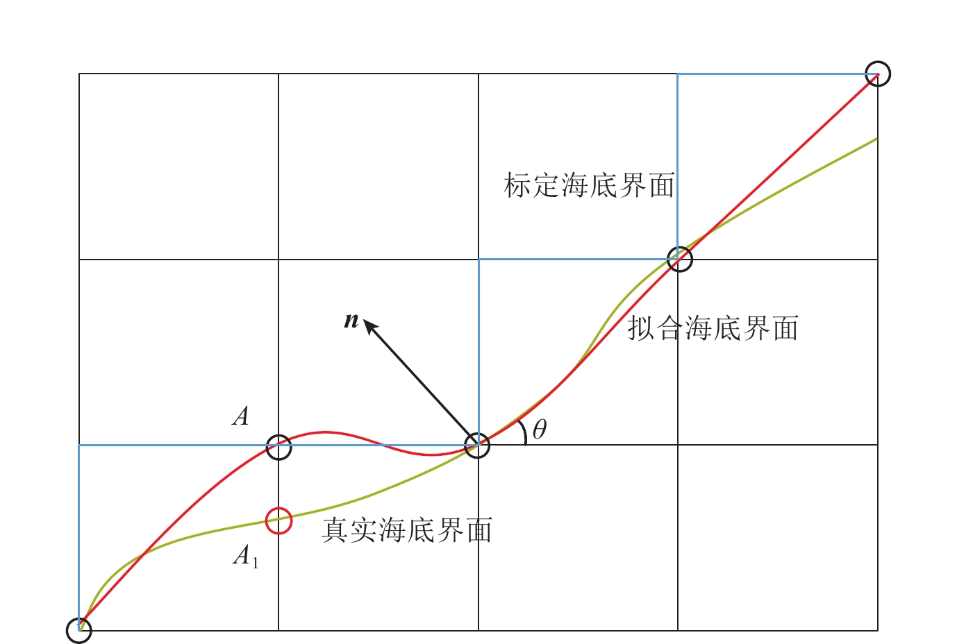
针对海底界面起伏的问题,本文采用三次样条海底界面定量表征方法,结合有限差分方法提出适用任意形状海底界面的地震波数值模拟方法. 如图8所示,黄色线条描述真实的海底,将海底深度对应标定在网格上,标定得到的海底界面会与真实界面有偏差,如图中用点A代替点A1. 对海底界面标定完毕后,作三次样条插值就可以得到光滑的海底界面(红色线条). 样条函数的导数即为θ的正切值,根据三角函数关系可以求出角度参数n=(nx,ny).
![]() 图 8 海底耦合边界的变角度处理Figure 8. Angle processing strategy of coupled boundary of the seabed
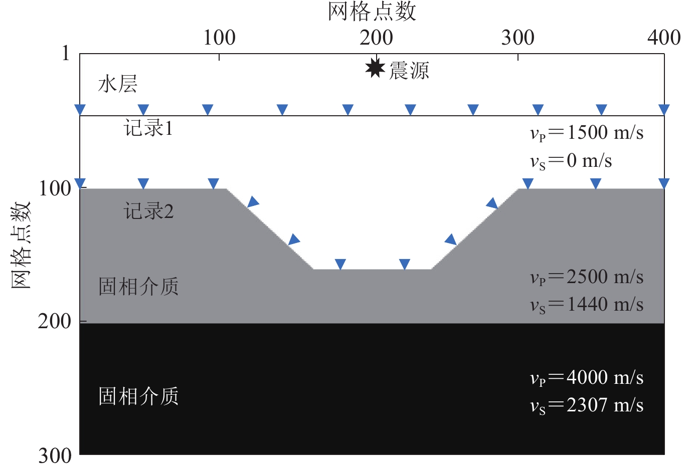
图 8 海底耦合边界的变角度处理Figure 8. Angle processing strategy of coupled boundary of the seabed检波器接收记录分为海中拖缆(记录1:拖缆水平置于海平面以下深度250 m处)和海底多分量(记录2)两种形式. 如图 9所示,采用拖缆接收得到的纯声波记录(图 9a)中可以清晰地看到入射P波,P−P反射波以及最下层界面产生的P−P−P反射波;在流固边界耦合介质记录(图 9b)中,由于介质物性的差异,海底P−P反射波能量很明显,透射波反射能量相对较弱.
![]() 图 9 凹陷模型拖缆接收共炮点记录(a) 纯声波记录;(b) 流固边界耦合记录;(c) 图(a)与图(b)中第200道记录的波形对比Figure 9. Common shot point records received by the streamer based on the sag model(a) Pure acoustic records;(b) Fluid-solid boundary coupled records;(c) Comparison of the 200th track records in Figs. (a) and (b)
图 9 凹陷模型拖缆接收共炮点记录(a) 纯声波记录;(b) 流固边界耦合记录;(c) 图(a)与图(b)中第200道记录的波形对比Figure 9. Common shot point records received by the streamer based on the sag model(a) Pure acoustic records;(b) Fluid-solid boundary coupled records;(c) Comparison of the 200th track records in Figs. (a) and (b)抽取图9a和图9b单炮记录中第200道进行波形对比,纯声波介质中可以清晰地识别入射P波,P−P反射波以及最下层界面产生的P−P−P反射波,而在流固边界耦合介质中,由于液相和固相介质的差异,加上转换波的产生,导致入射P波和海底P−P反射波能量很明显,而传入海底的透射波在海底物性差异分界面产生的反射能量很弱. 分析图9c可知:两介质中直达波基本吻合,地震波在海底界面发生反射并产生极性反转,海底为凹陷状,界面反射波来自不同方向,持续时间较长. 海底固相层界面产生的反射波在 1.1 s 左右接收,对于深层反射波的振幅相对比较弱.
如图10所示,采用海底多分量接收,纯声波介质(图10a)显示了入射P波和P−P反射波;水平分量(图10b)和垂直分量(图10c)波场快照显示了P−P,P−S和P−S−P反射波,剩余有效信息与层间多次波和转换波相互混叠. 抽取记录第150道,如图11圆圈圈出部分所示相位吻合. 通过对比凹陷模型3种波场(图12),可以看出本文提出的算法对于海底起伏界面的适应性良好.
![]() 图 11 纯声波介质与流固边界耦合介质多分量第150道记录对比曲线Figure 11. Comparison of the 150th record in pure-acoustic wave medium with that of multi-component records in fluid-solid coupled medium
图 11 纯声波介质与流固边界耦合介质多分量第150道记录对比曲线Figure 11. Comparison of the 150th record in pure-acoustic wave medium with that of multi-component records in fluid-solid coupled medium![]() 图 12 凹陷模型波场快照(a) 0.5 s时的纯声波波场;(b) 0.625 s时的应力-位移波场中的水平分量;(c) 0.75 s时的应力-位移波场中的垂直分量Figure 12. Snapshots of wavefield based on the sag model(a) Pure acoustic wavefield at the moment 0.5 s;(b) The horizontal component of stress-displacement wavefield at the moment 0.625 s;(c) The vertical component of stress-displacement wavefield at the moment 0.75 s
图 12 凹陷模型波场快照(a) 0.5 s时的纯声波波场;(b) 0.625 s时的应力-位移波场中的水平分量;(c) 0.75 s时的应力-位移波场中的垂直分量Figure 12. Snapshots of wavefield based on the sag model(a) Pure acoustic wavefield at the moment 0.5 s;(b) The horizontal component of stress-displacement wavefield at the moment 0.625 s;(c) The vertical component of stress-displacement wavefield at the moment 0.75 s![]() 图 10 凹陷模型海底多分量接收共炮点记录(a) 纯声波记录;(b) 水平分量记录;(c) 垂直分量记录Figure 10. Common shot point records of multi-component receiver based on the sag model(a) Pure acoustic records;(b) Horizontal component records;(c) Vertical component records
图 10 凹陷模型海底多分量接收共炮点记录(a) 纯声波记录;(b) 水平分量记录;(c) 垂直分量记录Figure 10. Common shot point records of multi-component receiver based on the sag model(a) Pure acoustic records;(b) Horizontal component records;(c) Vertical component records4. 讨论与结论
本文在推导任意形状下流固边界耦合条件的基础上,建立了地震波在流固耦合介质中传播的波动方程. 针对海底界面的不规则特点,在流固边界引入了方向因子,结合有限差分方法提出了对任意形状海底界面均适用的地震波数值模拟方法. 该方法既保留了有限差分剖分网格的规则化特点,又提高了对任意形状海底界面表征的精度. 在此基础上,为提高数值模拟精度,利用高阶空间差分方法压制了空间频散效应,提高了空间模拟精度,进一步利用波动方程将时间四阶微分算子转换至高阶的空间差分形式,提高了时间模拟精度和数值模拟的效率.
通过简单的层状模型和复杂模型验证了该方法的准确性和有效性. 该方法可以作为研究海洋地震勘探中地震波数值模拟方法的有力工具. 若遵循三维网格方法,本文推导的流固边界耦合介质高阶有限差分算法可以扩展到三维情况,同样可以适用于海洋环境逆时偏移和全波形反演.
-
![]()
图 1 流固耦合界面正应力连续
${n_x}, \ {n_y}, \ {n_z}$ 表示n与3个坐标轴夹角的余弦Figure 1. Fluid-solid coupling normal stress continuous in interface
${n_x}, \ {n_y}, \ {n_z}$ represents the cosine of the angle between the n and axis![]()
图 2 流固耦合分界面法向位移连续
Figure 2. Displacement continuous in normal direction at the fluid-solid coupling interface
![]()
图 3 时间二阶精度(a)和四阶精度(b)模拟的频散特性对比
Figure 3. Comparison of the dispersion properties of the second-order (a) and the fourth-order (b) time accuracy
![]()
图 5 水平层介质模型的共炮点地震记录
(a) 纯声波记录;(b) 水平分量记录;(c) 垂直分量记录
Figure 5. Common shot point seismic records based on horizontal layered medium model
(a) Pure acoustic records;(b) Horizontal component records;(c) Vertical component records
![]()
图 6 1 s (上)和1.2 s (下)时的水平层状介质模型波场
(a) 纯声波波场;(b) 应力-位移场中的水平位移分量;(c) 应力-位移场中的垂直位移分量
Figure 6. Snapshots of wavefields based on the horizontal layered medium model at the moment 1 s (upper panels) and 1.2 s (lower panels)
(a) Pure acoustic wavefield;(b) Horizontal displacement component of stress-displacement wavefield;(c) Vertical displacement component of stress-displacement wavefield
![]()
图 8 海底耦合边界的变角度处理
Figure 8. Angle processing strategy of coupled boundary of the seabed
![]()
图 9 凹陷模型拖缆接收共炮点记录
(a) 纯声波记录;(b) 流固边界耦合记录;(c) 图(a)与图(b)中第200道记录的波形对比
Figure 9. Common shot point records received by the streamer based on the sag model
(a) Pure acoustic records;(b) Fluid-solid boundary coupled records;(c) Comparison of the 200th track records in Figs. (a) and (b)
![]()
图 11 纯声波介质与流固边界耦合介质多分量第150道记录对比曲线
Figure 11. Comparison of the 150th record in pure-acoustic wave medium with that of multi-component records in fluid-solid coupled medium
![]()
图 12 凹陷模型波场快照
(a) 0.5 s时的纯声波波场;(b) 0.625 s时的应力-位移波场中的水平分量;(c) 0.75 s时的应力-位移波场中的垂直分量
Figure 12. Snapshots of wavefield based on the sag model
(a) Pure acoustic wavefield at the moment 0.5 s;(b) The horizontal component of stress-displacement wavefield at the moment 0.625 s;(c) The vertical component of stress-displacement wavefield at the moment 0.75 s
-
何燕. 2008. 正交各向异性弹性波高阶有限差分正演模拟研究[D]. 青岛: 中国石油大学(华东): 10–100. He Y. 2008. High-order Finite-Difference Forward Modeling of Elastic-Wave in Orthorhombic Aniostropic Media[D]. Qingdao: China University of Petroleum: 10–100 (in Chinese).
刘庆敏. 2007. 高阶差分数值模拟方法研究[D]. 青岛: 中国石油大学(华东): 6–15. Liu Q M. 2007. Method Study of High-Order Finite-Difference Numerical Modeling[D]. Qingdao: China University of Petroleum: 6–15 (in Chinese).
刘洋, 李承楚, 牟永光. 1998. 任意偶数阶精度有限差分法数值模拟[J]. 石油地球物理勘探, 33(1): 1–10. Liu Y, Li C C, Mou Y G. 1998. Finite-difference numerical modeling of any even-over accuracy[J]. Oil Geophysical Prospecting, 33(1): 1–10 (in Chinese).
吴国忱, 王华忠. 2005. 波场模拟中的数值频散分析与校正策略[J]. 地球物理学进展, 20(1): 58–65. Wu G C, Wang H Z. 2005. Analysis of numerical dispersion in wave-field simulation[J]. Progress in Geophysics, 20(1): 58–65 (in Chinese).
赵茂强. 2010. 多分量VSP/RVSP正演模拟方法研究[D]. 青岛: 中国石油大学(华东): 7–48. Zhao M Q. 2010. The Study of Multi-Component VSP/RVSP Seismic Forward Modeling[D]. Qingdao: China University of Petroleum: 7–48 (in Chinese).
Berenger J P. 1994. A perfectly matched layer for the absorption of electromagnetic waves[J]. J Comput Phys, 114(2): 185–200.
Cho Y, Ha W, Kim Y, Shin C, Singh S, Park E. 2016. Laplace–Fourier–domain full waveform inversion of deep-sea seismic data acquired with limited offsets[J]. Pure Appl Geophys, 173(3): 749–773.
Choi Y, Min D J, Shin C. 2008. Two-dimensional waveform inversion of multi-component data in acoustic-elastic coupled media[J]. Geophys Prospect, 56(6): 863-881.
Dablain M A. 1986. The application of high-order differencing to the scalar wave equation[J]. Geophysics, 51(1): 54–66.
Higdon R L. 1991. Absorbing boundary conditions for elastic waves[J]. Siam Journal on Numerical Analysis, 1991, 56(2): 231–241.
Levander A R. 1988. Fourth-order finite-difference P–SV seismograms[J]. Geophysics, 53(11): 1425–1436.
Lee H Y, Lim S C, Min D J, Kwon B D, Park M. 2009. 2D time-domain acoustic-elastic coupled modeling: A cell-based finite-difference method[J]. Geosci J, 13(4): 407–414.
Madariaga R. 1976. Dynamics of an expanding circular fault[J]. Bull Seismol Soc Am, 66(3): 639–666.
Reynolds A C. 1978. Boundary conditions for the numerical solution of wave propagation problems[J]. Geophysics, 43(6): 1099–1110.
Virieux J. 1986. P-SV wave propagation in heterogeneous media: Velocity-stress finite-difference method[J]. Geophysics, 51(4): 889–901.
Yu P F, Geng J H, Li X B, Wang C L. 2016. Acoustic-elastic coupled equation for ocean bottom seismic data elastic reverse time migration[J] Geophysics, 81(5): S333–S345.
Zhang J F. 2004. Wave propagation across fluid–solid interfaces: A grid method approach[J]. Geophys J Int, 159(1): 240–252.
-
期刊类型引用(6)
1. 段沛然,谷丙洛,李振春,李青阳. 起伏地表QR径向基函数有限差分及其在弹性波逆时偏移中的应用. 地球物理学报. 2024(03): 1181-1207 .  百度学术
百度学术
2. Mu-Ming Xia,Hui Zhou,Chun-Tao Jiang,Han-Ming Chen,Jin-Ming Cui,Can-Yun Wang,Chang-Chun Yang. Wave propagation across fluid-solid interfaces with LBM-LSM coupling schemes. Petroleum Science. 2024(05): 3125-3141 . 必应学术
3. 陈苏,丁毅,孙浩,赵密,王进廷,李小军. 物理驱动深度学习波动数值模拟方法及应用. 力学学报. 2023(01): 272-282 . 百度学术
4. 李广才,王兴宇,李培,张鹏辉,何梅兴. 地震正演模拟技术在膏盐岩识别中的应用. 中国煤炭地质. 2023(02): 67-72 . 百度学术
5. 刘家豪,雍凡,刘振东,张辉,严加永,阮小敏,高凤霞,陈昌昕. 江南造山带中段地壳结构特征——来自武宁—吉安深反射地震随机介质相关长度分析的认识. 地球学报. 2022(06): 803-816 . 百度学术
6. 刘立彬,段沛然,张云银,田坤,谭明友,李振春,窦婧瑛,李青阳. 基于无网格的地震波场数值模拟方法综述. 地球物理学进展. 2020(05): 1815-1825 . 百度学术
其他类型引用(7)
 下载:
下载:


计量
- 文章访问数: 1538
- HTML全文浏览量: 953
- PDF下载量: 89
- 被引次数: 13
