

Research on the static-dynamic boundary switch and its rationality verification method
-
摘要:
繁琐复杂的静动力边界转换处理是进行静动力耦合模拟的关键步骤,为了研究黏弹性边界条件下传统静动力边界转换的合理性及其验证方法的适用性,本文首先根据弹性叠加原理提出了一种验证静动力耦合模拟分析中静动力边界转换合理性的方法(参考解法);然后基于有限元软件ABAQUS,并结合自行研发的适用于成层介质的黏弹性边界施加和等效节点力计算程序VBEA2.0,对多土层自由场静动力耦合模型和土-地下结构静动力耦合模型进行了地震反应分析,对参考解法的适用性进行了探究;最后使用本文提出的参考解法,对一种典型的未进行合理静动力边界转换的自由场模型进行了分析,探讨了静动力边界转换产生振荡的原因和机理。研究结果表明:用于验证静动力边界转换合理性的参考解法,既适用于多土层自由场静动力耦合计算模型,又适用于土-结构相互作用的静动力耦合模型;静动力边界转换后产生的振荡是静动力耦合计算模型静力不平衡所导致,一般是因为未合理施加边界反力或单元应力。
Abstract:In the dynamic analysis of underground structure subjected to seismic loading, dynamic boundary (e.g., viscous-spring boundary condition, transient wave transmission boundary, etc.) is essential to be adopted to absorb the reflected wave. Generally, the dynamic boundary is not applicable to the static analysis in the simulation of seismic response of underground structure. Taking the viscous-spring boundary condition as an example, if this dynamic boundary condition is applied during the static analysis phase the subsequent dynamic response will be significantly affected, since this operation results in incorrect input of ground motion in the numerical model. To solve this problem, the traditional approach involves employing a fixed boundary during static analysis, which is then replaced by a dynamic boundary during dynamic analysis. Specifically, the dynamic calculation is performed using a viscous-spring boundary condition based on the results obtained in the static analysis with static boundary condition. The complex process of switching between static and dynamic boundary is a significant step in the static-dynamic coupling simulation. However, oscillations occur at the onset of dynamic response when switching from a static to a dynamic boundary, affecting dynamic response of acceleration, velocity, displacement, etc. To investigate the validity of the traditional scheme for switching static-dynamic boundary condition types (from static boundary to viscous-spring boundary) and the applicability of the verification method the following works were conducted: based on the superposition principle, a method for verifying the rationality of static-dynamic boundary switch is given (reference method). Using the finite element method software ABAQUS and the self-developed VBEA2.0 program, which can automatically set viscous-spring boundary and input seismic wave, the seismic response of layered free field and soil-underground structure models (Dakai metro station) considering integral static-dynamic analysis are analyzed. Based on these results, the applicability of the reference method is discussed. Adopting this reference method, an analysis is conducted on a free field model employing a typical, unreasonable static-dynamic switching method with the aim of shedding lights on the oscillations during the switching between the static and dynamic boundary condition. Finally, a potential mechanism for the observed oscillation in the process of switching boundary condition is proposed. The simulation results indicate that the introduced method of switching boundary conditions for the viscous-spring boundary condition in seismic analysis performs well, effectively avoiding oscillations at the beginning of dynamic analysis. The procedure should be as follows: First, perform the static analysis to balance the in-situ stress; then, carry out the switching between static and dynamic boundaries; and finally, calculate the dynamic analysis. In particular, the rational application of nodal reaction force, gravity, and element stress is a key factor influencing the rationality of static-dynamic boundary switching.In addition to that, the proposed reference method for verifying the rationality of static-dynamic boundary switching is applicable to both the layered free field model and the soil-underground structure model based on the seismic response of the free field and the field embedding an underground structure. In the reference method, dynamic results of the elastic and non-damped model, without considering the static-dynamic coupling effects (reference model), are used as the benchmark solution for checking the dynamic response analysis. Dynamic response of the numerical model with the correct static and dynamic boundary switching should align with the corresponding dynamic response recorded in the reference model, in terms of acceleration, displacement time history. The second-order Euclidean norm is recommended for calculating the relative errors between the benchmark model and the numerical model which needs to check the validity of the traditional scheme for switching static-dynamic boundary. This can intuitively indicate the presence of oscillations in the early stage of dynamic calculation and assess the degree of their impact on the later stage, offering an effective tool to examine the rationality of static and dynamic boundary switching for a reasonable static-dynamic coupling analysis of soil-underground structure. Lastly, to reveal the mechanism of oscillation in the switching process of static and dynamic boundary, a model with only nodal reaction forces on the truncated boundary extracted and applied for the dynamic phase, which is typically incorrect to switch the static boundary condition to dynamic boundary condition, is built and analyzed. This incorrect way generates substantial forces in the spring elements leading the inaccurate seismic wave input employing equivalent nodal forces in the dynamic phase, according to the magnitude of elastic fore for spring elements located at the viscous-spring boundary. This means the numerical model may underestimate the dynamic response as portion of the equivalent nodal forces are counteracted by these forces from the springs. Therefore, the oscillated response in this switching procedure of static-dynamic boundary is typically caused by the non-static equilibrium in the static-dynamic coupling calculation model, possibly resulting from incorrect static-dynamic boundary switching.
-
引言
岩土及地下结构的静动力耦合模拟直接影响着其地震反应的合理性。在考虑土体重力引起的初始应力和地震动力作用的静动力耦合地震动力反应分析中,静力计算采用的是静力边界,如固定边界、滚轴边界等;有别于静力分析,动力计算使用的是动力边界,如透射边界(廖振鹏等,1984)、无限元边界(Ungless,1973)、黏弹性边界(Deeks,Randolph,1994)等。一般的动力边界不能用于静力分析,于是数值模拟计算过程中出现了边界不统一的矛盾。以黏弹性边界为例,若在静力分析中使用常规黏弹性动力边界,会影响后续动力反应(郭亚然等,2018)。为解决这一问题,目前发展了三类方法。第一类是实现静动力耦合分析时边界条件的统一性,将动力边界用于静力分析中。此类方法利用了黏弹性边界良好的鲁棒性,通过修正弹性系数Kb来发展静动力统一边界。刘晶波和李彬(2005)提出了一种三维黏弹性静动力统一人工边界以解决静动力耦合动力分析中静动力边界不统一的问题,但此种边界在静力计算时模拟结果存在一定误差(高峰,赵冯兵,2011)。廖维张等(2006)提出了一种开放系统非线性动力反应分析算法,在进行地下结构非线性动力地震反应分析时,将无零频限制的黏弹性边界用于静力分析中,以此实现静动力边界条件的统一。第二类方法是采用动力学解法计算静力反应(杜修力等,2000)。此方法将静力荷载视为零荷载时刻所施加的阶跃荷载,以阶跃函数的形式施加在结构上,用动力方法进行计算,由于模型阻尼的作用,阶跃荷载引起的动力反应会很快衰减并处于平衡状态,然后再进行动力计算分析。第三类处理静动力边界矛盾的传统方法是静动力边界转换方法。此方法在静力计算完成后,将静力边界转换成动力边界,再进行动力计算。具体来讲,先用固定边界计算重力引起的单元应力和边界节点反力,以此作为动力分析的初始条件,最后进行地震动力分析。
使用这种传统的静动力边界转换方法来进行地震动力反应数值模拟比较普遍,但是静动力边界转换的处理细节不尽相同(高峰,赵冯兵,2011;王苏等,2012;付培帅,2015;郭亚然等,2018),且转换过程中静力边界转换成动力边界时模型会出现振荡反应(Su et al,2021)。Su等(2021)提出利用ABAQUS中生死单元功能来杀死和激活黏弹性边界(弹簧和阻尼单元)以实现静动力边界的切换,但未解释振荡的原因和机理。王苏等(2012)给出了静动力边界转换的分析思路。高峰和赵冯兵(2011)针对静动力边界转换方法开展了相应的工作,提出了一种验证静动力人工边界转换合理性的方法,但不能直观地反应出静动力边界转换结果对后续动力计算的影响。
静动力边界转换过程较为繁琐,涉及到应力的提取和施加,静动力边界的切换以及地震动的输入,人为操作过程中容易出错,出现振荡反应,因此有必要在进行动力分析前对静动力边界转换的合理性进行检验。为此,本文将围绕静动力边界转换中出现的振荡问题及转换合理性验证方法开展相关研究工作:根据岩土材料的特性提出参考解法,并通过算例对该方法的适应性进行探讨,以验证静动力边界转换的合理性;通过对算例的分析揭示振荡的原因和机理,以加深对边界转换过程中振荡的理解。
1. 地震动垂直入射黏弹性边界
黏弹性边界是众多动力边界中的一种,其本质是为了保证计算区域内反射波和散射波在边界上不发生反射,方法是在截断的模型边界上施加连续的并联弹簧和阻尼器。弹簧刚度系数和阻尼系数由下式获得(刘晶波等,2007):
$$ \left\{ \begin{array}{l} {K_{{\rm{BT}}}} = {\alpha _{\rm{T}}}\dfrac{G}{R},{C_{{\rm{BT}}}} = \rho {C_{\rm{S}}} \text{,} \\ {K_{{\rm{BN}}}} = {\alpha _{\rm{N}}}\dfrac{G}{R},{C_{{\rm{BN}}}} = \rho {C_{\rm{P}}} \text{,} \end{array} \right. $$ (1) 式中:$ K_{{\rm{BT}}} $和$ K_{{\rm{BN}}} $分别为切向弹簧和法向弹簧的刚度系数;$ C_{{\rm{BT}}} $和$ C_{{\rm{BN}}} $分别为切向阻尼器和法向阻尼器的阻尼系数;$ \alpha_{{\rm{T}}} $和$ {\alpha}_{{\rm{N}}} $为黏弹性边界的修正系数,二维情况下,$ \alpha_{{\rm{T}}} $和$ {\alpha}_{{\rm{N}}} $的建议取值为$ \alpha_{{\rm{T}}}=0.5 $,$\alpha_{{\rm{N}}}=1$ (刘晶波等,2007);R为波源至人工边界点的距离;$\; \rho $和G分别为介质的密度和剪切模量;$ C_{{\rm{S}}} $和$ C_{{\rm{P}}} $分别为介质的剪切波速和纵波波速。各边界节点地震动等效节点力计算公式如式(2)—(5)所示。本文在马笙杰等(2020)和马笙杰(2021)文献基础上,进一步编制了适用于成层介质的等效节点力计算及黏弹性边界施加的程序VBEA2.0(program for viscous-spring boundary and equivalent nodal load application 2.0),以实现地震动在黏弹性边界上的垂直入射。等效节点力Fb的计算方法为
$$ {F_{{\rm{b}}}}= ( {K_{{\rm{}}b}} {{\boldsymbol{u}_{{\rm{b}}}}}+{{C_{{\rm{b}}}} {{\dot{\boldsymbol{u}}}}_{{\rm{b}}}}+{{\sigma_{{\rm{b}}}} {\boldsymbol{n}}} ) { A_{{\rm{b}}} }\text{,} $$ (2) 底边界,
$$ \left\{\begin{aligned} F_{{\rm{b}} x}^{-y}= & A_{{\rm{b}}}\left[K_{\mathrm{BT}} {\boldsymbol{u}} ( t ) +C_{\mathrm{BT}} \dot{{\boldsymbol{u}}} ( t ) - \frac{G}{{\rm{d}} y} ( {\boldsymbol{u}}_{x}^{i}-{\boldsymbol{u}}_{x}^{j} ) -\frac{1}{2} \rho {\rm{d}} y \ddot{{\boldsymbol{u}}}_{x}^{j}\right] \\ F_{{\rm{b}} y}^{-y}= & 0\text{,} \end{aligned}\right. \text{,} $$ (3) 左边界,
$$ \left\{\begin{array}{l} F_{{{\rm{b}}x}}^{-x}=A_{{\rm{b}}} [ K_{\mathrm{BN}} {\boldsymbol{u}} ( t ) +C_{\mathrm{BN}} \dot{{\boldsymbol{u}}} ( t ) ] \text{,} \\ F_{{\rm{b}} y}^{-x}=-A_{{\rm{b}}}\left[\dfrac{G}{{\rm{d}} y} ( {\boldsymbol{u}}_{x}^{i}-{\boldsymbol{u}}_{x}^{j} ) +\dfrac{1}{2} \rho {\rm{d}} y \ddot{{\boldsymbol{u}}}_{x}^{j}\right]\text{,} \end{array}\right. $$ (4) 右边界,
$$ \left\{\begin{array}{l} F_{{{\rm{b}}x}}^{x}=A_{{\rm{b}}} [ K_{\mathrm{BN}} {\boldsymbol{u}} ( t ) +C_{\mathrm{BN}} \dot{{\boldsymbol{u}}} ( t ) ] \text{,} \\ F_{{\rm{b}} y}^{x}=A_{{\rm{b}}}\left[\dfrac{G}{{\rm{d}} y} ( {\boldsymbol{u}}_{x}^{i}-{\boldsymbol{u}}_{x}^{j} ) +\dfrac{1}{2} \rho {\rm{d}} y \ddot {\boldsymbol{u}}_{x}^{j}\right]\text{,} \end{array}\right. $$ (5) 式中:$K_{\rm{b}} {\boldsymbol{u}}_{\rm{b}}$表示为了克服位移引起弹簧单元所产生的附加应力;$C_{\rm{b}} \dot{{\boldsymbol{u}}}_{\rm{b}}$表示为了克服速度引起阻尼器产生的附加应力;$\sigma_{\rm{b}} {\boldsymbol{n}}$为自由场地震动在边界产生的应力张量;${\boldsymbol{u}}_{\rm{b}}= [ \begin{array}{lll}u & v & w\end{array} ] ^{\mathrm{T}}$为入射波位移向量;$\dot {\boldsymbol{u}}_{\rm{b}}= [ \begin{array}{lll}\dot u & \dot v & \dot w\end{array} ] ^{\mathrm{T}}$为入射波速度向量;Ab为边界节点控制面积,二维模型中为节点控制边长;n为边界外法线方向余弦向量;二维情况下,边界节点入射波位移向量为${\boldsymbol{u}}_{\rm{b}}= [ u \;\;v ] ^{\mathrm{T}}$,入射波速度向量为$\dot {\boldsymbol{u}}_{\rm{b}}= [ \dot u \;\;\dot v ] ^{\mathrm{T}}$;$K_{\rm{b}}$,$ C_{\rm{b}} $分别为黏弹性边界上弹簧刚度系数和阻尼系数。
2. 验证静动力边界转换合理性的方法
2.1 静动力边界转换方法
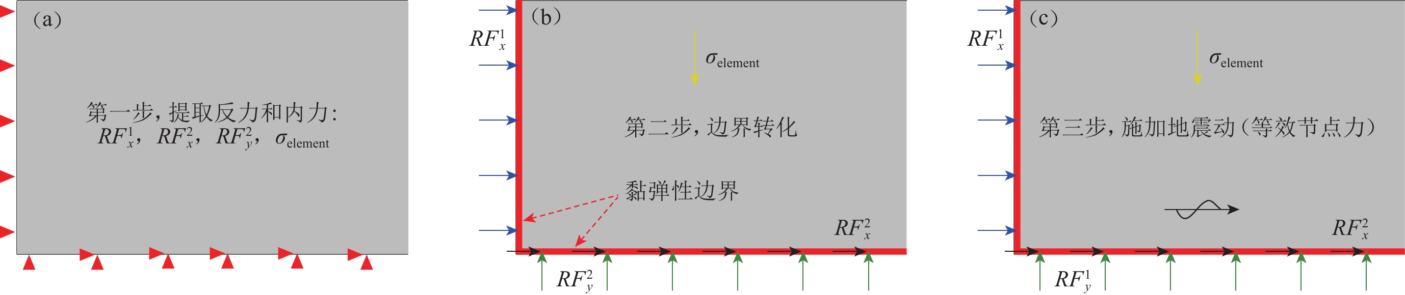
本文采用如下静动力边界转换方法来进行静动力耦合计算:先用固定边界计算由重力引起的单元应力和边界节点反力,以此作为动力分析的初始条件;然后进行地震动力分析,即先进行地应力平衡计算,再进行静动力边界转换,最后进行地震动力计算。具体过程如图1所示:
![]() 图 1 静动力边界转换方法示意图(a) 地应力平衡;(b) 静动力边界转化;(c) 施加地震荷载Figure 1. Schematic diagram of static-dynamic boundary switch(a) In-situ stress balance;(b) Switching between static and dynamic boundary;(c) Application of earthquake loading
图 1 静动力边界转换方法示意图(a) 地应力平衡;(b) 静动力边界转化;(c) 施加地震荷载Figure 1. Schematic diagram of static-dynamic boundary switch(a) In-situ stress balance;(b) Switching between static and dynamic boundary;(c) Application of earthquake loading1) 首先约束模型侧边界水平方向、底部水平及竖向位移,施加重力,通过静力分析进行地应力平衡,使模型的初始位移为零,一般10−5即满足要求。提取侧边界节点的水平反力$ R F_{x}^{1} $、底部节点的水平反力$ R F_{x}^{2} $和竖向反力$ R F_{y}^{2} $以及模型所有单元的应力$ \sigma $。其中反力RF (reaction force)的下标表示力的方向,上标1表示侧边界,上标2表示底边界。对于二维问题,$ \sigma $为在ABAQUS中提取的积分点(centroid)应力分量S11,S22,S33,S12,对于三维问题,还应提取S13和S23。
2) 对地下结构地震反应分析模型施加黏弹性边界,取消1)中静力边界条件并施加地应力平衡后获得的边界节点反力、所有单元应力和重力,以此实现静动力边界的转换。
3) 在前面静力分析步的基础上创建隐式动力分析步,并在该分析步施加地震等效节点力和重力荷载。
2.2 参考解法
由2.1节可知,静动力转换过程较为繁琐,需要人为操作的步骤较多,因此在进行动力分析前有必要进行边界转换成功与否的验证,以保证后续动力分析计算的正确性。高峰和赵冯兵(2011)提出施加零动力荷载的方法来检验静动力人工边界转换误差。零动力荷载法能观察到地震动力反应时程曲线(位移、应力等)的初期是否有波动,但不能直观反映此波动的相对大小以及对后续地震动力反应的影响程度。本文中的参考解法能够直接得到静动力边界转换后与参考解的误差数值,为合理判断静动力边界合理转换提供一种有效的方法。
根据弹性叠加原理,现给出一种判断静动力边界转换合理性方法:参考解法。由该原理可知,在线弹性无阻尼条件下,考虑静动力耦合与不考虑静动力耦合的自由场场地地震动力计算模型在各深度处的地震动力反应(加速度时程、位移时程等)是一致的。因此可以把不考虑静动力耦合的模型计算结果作为动力反应分析的参考解来判断静动力边界转换的正确性,这样就能直接得出静动力耦合计算模型在静边界转换后计算结果与理论值之间的误差,可以确保后续非线性静动力耦合模拟的合理性和正确性。具体方法如下:先建立不施加重力引起的初始应力的自由场弹性计算模型(不考虑静动力耦合作用的计算模型),施加地震动力荷载,进行动力分析;另外建立一个施加重力引起的初始应力并进行静动力边界转换的弹性计算模型(考虑静动力耦合作用的计算模型),然后施加同样的地震动力荷载,进行动力分析。通过比较两模型在各深度处地震动力反应(位移、加速度时程),即可判断考虑静动力耦合模型的静动力边界转换是否合理,若两者同一模型位置处的位移、加速度时程等动力反应一致,则静动力边界转换合理;反之,不合理。在具体操作过程中,建议选取侧边界底部、顶部节点以及模型中部、顶部和底部的节点的加速度动力响应来比较验证,具体原因将在第4节讨论。
3. 参考解法适用性探究
3.1 成层自由场静动力耦合计算模型
3.1.1 计算模型
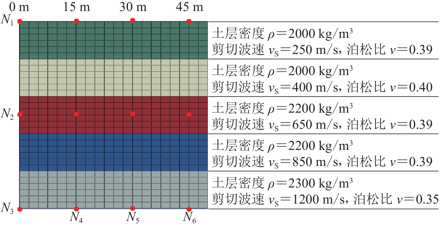
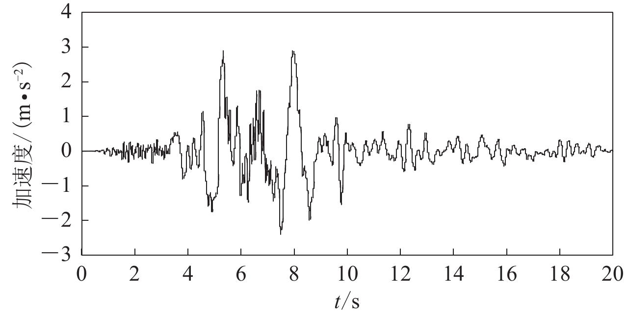
建立两类不同土层厚度的成层自由场模型(100 m×50 m和200 m×100 m),模型都均分为5层土层且两个模型都使用图2中的材料参数。不考虑土体的阻尼,采用弹性本构模型来描述土层的地震动力反应。有限元网格尺寸只有足够小,高频的地震波才能在离散体系中传播,进而保证计算精度。要获得波长为$ \lambda_{T} $波动的可靠数值结果,网格尺寸$ \Delta x $应当满足式(廖振鹏,刘晶波,1986):$\Delta x {\text{≤}}$(1/10—1/8)λT,本研究中采用0.5 m的四节点应变单元(CPE4)对模型进行离散。两种不同尺寸的模型分别考虑施加重力引起的初始应力(考虑静动力耦合作用)和不考虑施加初始应力(不考虑静动力耦合作用),一共4种不同计算工况。使用适用于成层地基的黏弹性边界施加和地震输入程序VBEA2.0,在模型两侧、底部施加黏弹性边界和等效节点力,将计算模型考虑为柔性地基,即:在地震波输入后,计算区域内的反射波和散射波不会在边界上发生反射。输入的地震动为神户海洋气象台处获得的地震南北分量前20 s地震动记录作为模型的输入,如图3所示。
![]() 图 3 日本神户地震南北分量加速度时程Figure 3. Acceleration time history of the north and south components of the Kobe earthquake
图 3 日本神户地震南北分量加速度时程Figure 3. Acceleration time history of the north and south components of the Kobe earthquake3.1.2 计算结果分析
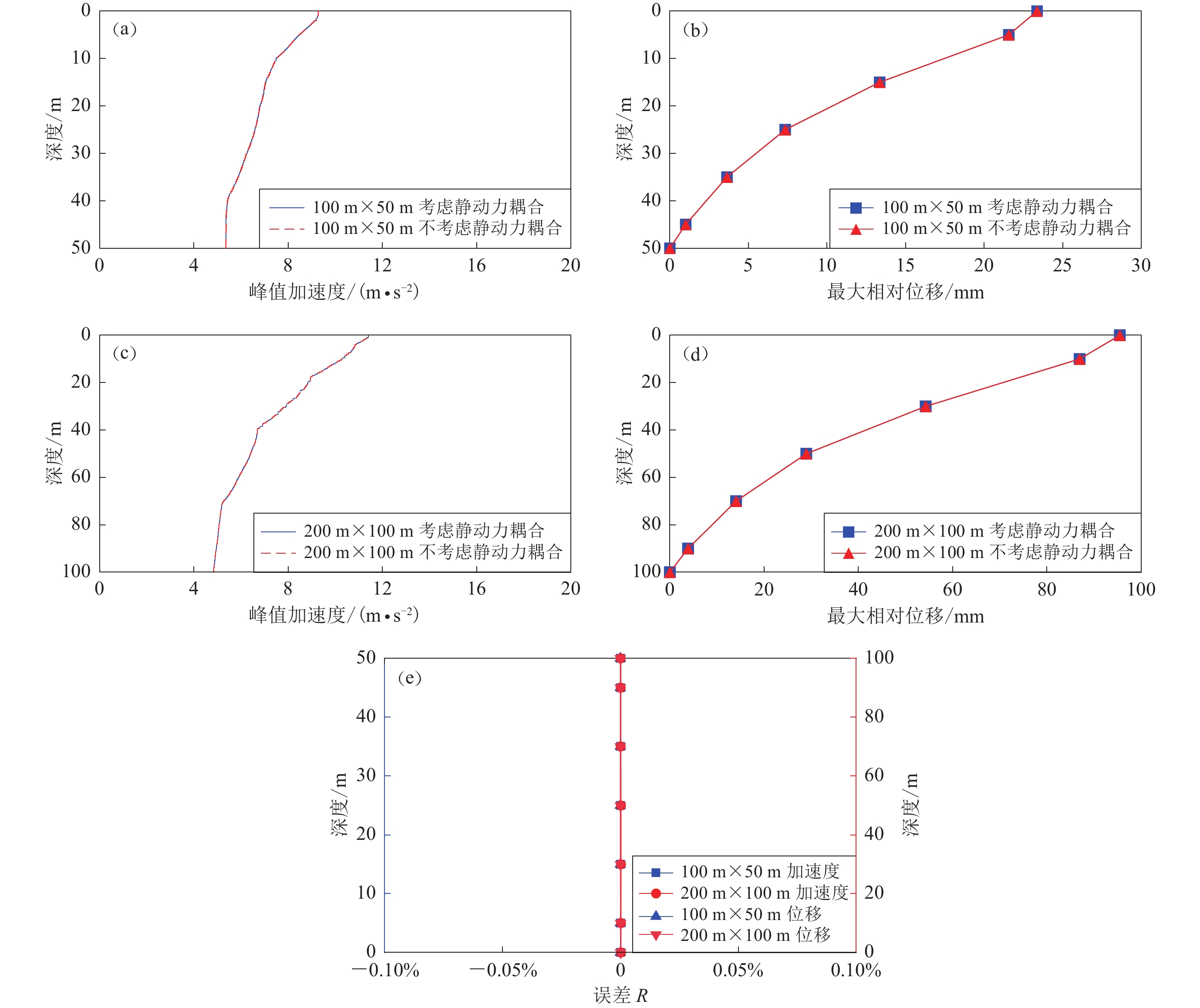
在不同工况下两种不同尺寸模型的中部沿深度方向的地震反应计算结果如图4所示。由图4a和4b可知,50 m高的多土层自由场模型在地震作用下,考虑静动力耦合作用和不考虑静动力耦合作用两种工况下,随深度变化的峰值加速度和最大相对位移曲线吻合得很好。对于100 m高的多土层自由场模型,土层各深度节点峰值加速度以及最大相对位移的趋势与50 m高的自由场模型相似,考虑静动力耦合作用和不考虑静动力耦合工况的加速度、位移动力计算结果是一致的,也吻合得很好,如图4c和4d所示。
![]() 图 4 自由场地震反应计算结果(a) 100 m×50 m模型峰值加速度;(b) 100 m×50 m模型最大相对位移;(c) 200 m×100 m模型峰值加速度;(d) 200 m×100 m模型最大相对位移;(e) 随深度变化的加速度、位移时程误差Figure 4. Seismic dynamic response of free field(a) Maximum acceleration for 100 m×50 m model;(b) Maximum relative displacement for 100 m×50 m model;(c) Maximum acceleration for 200 m×100 m model;(d) Maximum relative displacement for 200 m×100 m model;(e) Acceleration and displacement time-history errors with varying depths
图 4 自由场地震反应计算结果(a) 100 m×50 m模型峰值加速度;(b) 100 m×50 m模型最大相对位移;(c) 200 m×100 m模型峰值加速度;(d) 200 m×100 m模型最大相对位移;(e) 随深度变化的加速度、位移时程误差Figure 4. Seismic dynamic response of free field(a) Maximum acceleration for 100 m×50 m model;(b) Maximum relative displacement for 100 m×50 m model;(c) Maximum acceleration for 200 m×100 m model;(d) Maximum relative displacement for 200 m×100 m model;(e) Acceleration and displacement time-history errors with varying depths为进一步确定静动力耦合作用对自由场地震动力反应的影响,采用二阶欧几里得范数来量化和分析自由场模型中部沿深度方向节点的加速度时程误差值,如式(6)所示。
$$ R=\frac{\|X-Y\|^{2}}{\|Y\|^{2}}=\frac{\sqrt{\displaystyle\sum_{i=1}^{n}\left|x_{i}-y_{i}\right|^{2}}}{\sqrt{\displaystyle\sum_{i=1}^{n}\left|y_{i}\right|^{2}}} {\text{×}} 100 \text{%} \text{,} $$ (6) 式中,X为未考虑静动力耦合作用的加速度时程计算结果,Y表示考虑静动力耦合作用的加速度时程计算结果,将其作为参考解。图4e给出了两种不同尺寸模型不考虑静动力耦合作用时,误差随深度变化的曲线,可以看出,四个算例模型中部沿深度方向节点的加速度和位移时程误差都接近于零。
综合上述结果,在黏弹性边界下,弹性模型考虑静动力耦合作用与否,不影响模型各深度的峰值加速度、相对最大位移的动力计算结果。因此,在弹性自由场静动力耦合计算模型中,把不考虑静动力耦合作用的计算模型的动力反应结果作为参考解来判断静动力边界转换的合理性和正确性是可行的。
3.2 土-地下结构静动力耦合计算模型
3.2.1 计算模型
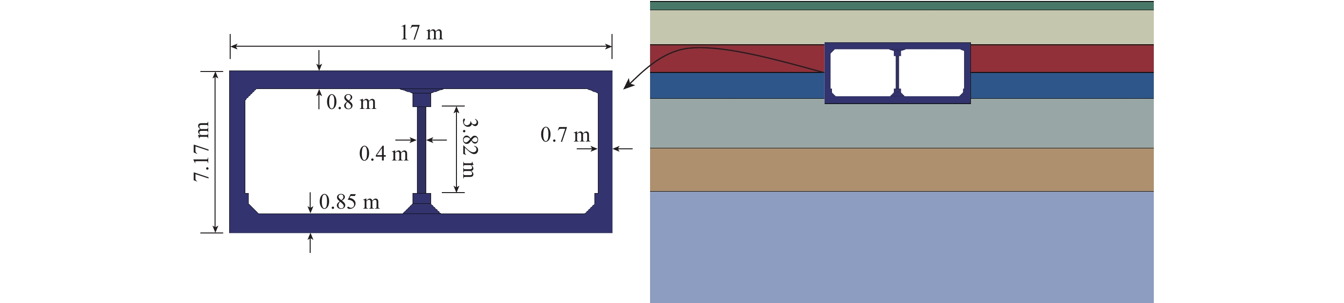
本节以日本大开地铁车站及其场地条件(曹炳政等,2002)作为研究对象,并以其为基准,通过调整土层剪切波速来获得另外较软地层和较硬地层场地,以此建立三种不同坚硬程度土层的弹性土-地下结构静动力耦合计算模型,场地条件如表1所示。车站主体为C30混凝土,将其考虑为线弹性,弹性模量为$ 3 {\text{×}} 10^{4}\; \mathrm{MPa} $,泊松比为0.18,密度为2 500 kg/m3,采用等效前、后刚度不变原则,把中柱弹性模量折减为$ 0.857 {\text{×}} 10^{4}\; \mathrm{MPa} $ (陈国兴,2007)。土-地下结构静动力耦合有限元模型宽为120 m,高为42 m,在基岩下20 m处截断,如图5所示。不考虑土与结构之间地震荷载所导致的错动、滑移等现象,仅考虑它们之间完全黏结的情况,即:使用绑定约束(Tie约束)。使用自编的程序VBEA2.0实现地震动从模型底部垂直输入,输入的地震动加速度时程与4.1节一致,如图3所示。
表 1 大开地铁车站数值模型场地条件参数Table 1. Mechanical parameters of the soil layers for the Dakai metro station土质 模型各层厚度/m 密度/(kg·m−3) 较软地层模型vS
/(m·s−1)真实地层模型vS
/(m·s−1)较硬地层模型vS
/(m·s−1)泊松比 人工填土 1 1 900 80 140 290 0.333 全新世砂土 4 1 900 80 140 290 0.320 全新世砂土 3 1 900 110 170 320 0.320 更新世黏土 3 1 900 130 190 340 0.400 更新世黏土 6 1 900 180 240 390 0.300 更新世砂土 5 2 000 270 330 480 0.260 基岩 20 2 000 1 000 1 000 1 000 0.260 3.2.2 计算结果分析
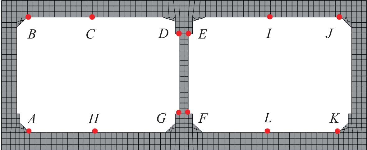
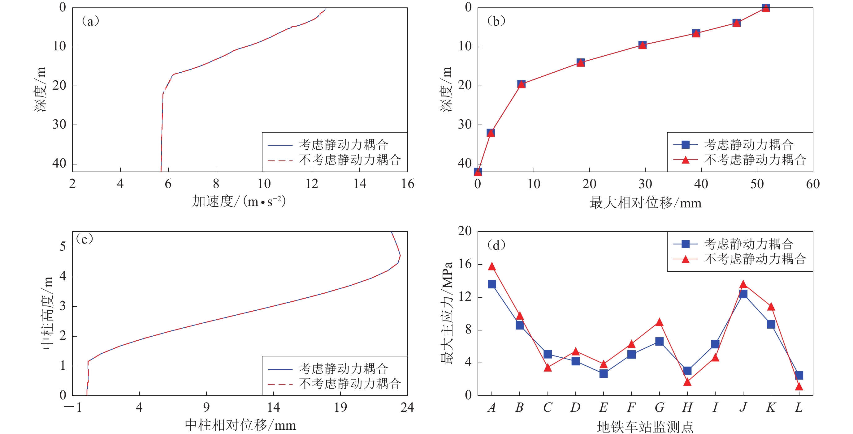
选取车站结构中柱和距车站右侧墙3.5 m处土层的水平峰值加速度和水平最大相对位移,以及车站结构重要位置处的最大主应力来反映结构和地基土的地震响应。上述数据均取地震动力分析时程中绝对值的最大值。结构重点位置监测点设置如图6所示。
根据大开车站真实地层模型计算获得的考虑和不考虑静动力耦合作用下的地震动力反应结果对比如图7所示。分析可知,大开车站场地模型在考虑和不考虑静动力耦合作用的情况下,地基土随深度变化的峰值加速度和最大相对位移几乎完全一致,车站中柱的最大相对位移在两种情况下也吻合得很好,而车站结构关键点的最大主应力也有类似的结果,在数值上相差不大。图8给出了真实地层工况下合理进行静动力边界转换后,模型左边界顶、底部节点及模型中部顶点及底边节点的水平方向加速度时程和位移时程曲线,可以看出各时程前段均未出现振荡。软弱地层模型和较硬地层模型计算结果与上述真实地层模型相似,其场地土和中柱的地震动力反应在考虑和不考虑静动力耦合的作用下差别不大,由于篇幅原因不再给出其具体结果。
![]() 图 7 带地下结构的成层场地地震动力反应计算结果(a) 场地土PGA;(b) 场地土最大相对位移;(c) 车站中柱最大相对位移;(d) 车站结构重要部位最大主应力Figure 7. Earthquake dynamic response of underground structure in the layered site(a) Maximum acceleration of the site;(b) Maximum relative displacement of the site;(c) Maximum relative displacement of the central column;(d) Maximum principal stress at points in the station
图 7 带地下结构的成层场地地震动力反应计算结果(a) 场地土PGA;(b) 场地土最大相对位移;(c) 车站中柱最大相对位移;(d) 车站结构重要部位最大主应力Figure 7. Earthquake dynamic response of underground structure in the layered site(a) Maximum acceleration of the site;(b) Maximum relative displacement of the site;(c) Maximum relative displacement of the central column;(d) Maximum principal stress at points in the station![]() 图 8 带地下结构的成层场地左边界及中部节点水平向的加速度时程(左)和位移时程(右)(a) 左边界顶部节点;(b) 地表中部节点;(c) 左边界底部节点;(d) 底边界中部节点Figure 8. Horizontal acceleration (left) and displacement (right) time history of nodes at the left boundary and the vertical middle of underground structure in the layered site(a) Node at the top of the left boundary;(b) Node at the centre of the surface;(c) Node at the bottom of the left boundary;(d) Node at the centre of the base
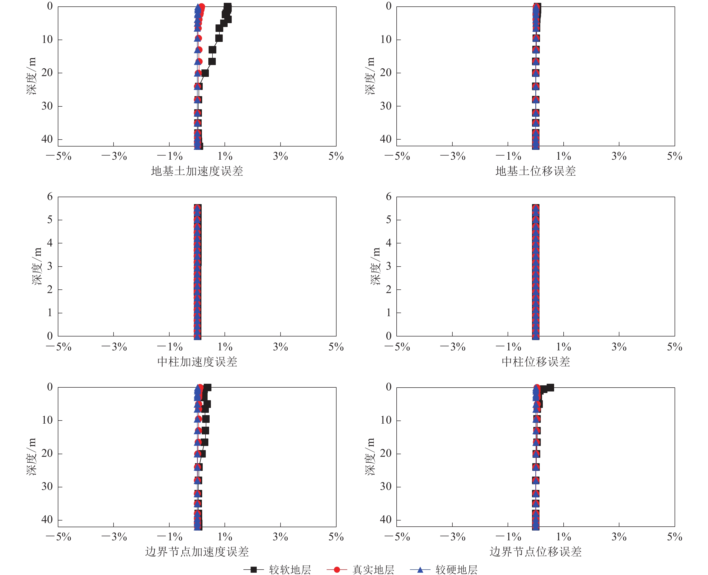
图 8 带地下结构的成层场地左边界及中部节点水平向的加速度时程(左)和位移时程(右)(a) 左边界顶部节点;(b) 地表中部节点;(c) 左边界底部节点;(d) 底边界中部节点Figure 8. Horizontal acceleration (left) and displacement (right) time history of nodes at the left boundary and the vertical middle of underground structure in the layered site(a) Node at the top of the left boundary;(b) Node at the centre of the surface;(c) Node at the bottom of the left boundary;(d) Node at the centre of the base为进一步研究静动力耦合作用的影响对土-地下结构计算模型的影响,利用二阶欧几里得范数(式(6))计算以比较这些模型的边界节点、地基土和结构中柱在考虑静动力耦合作用时得到的加速度时程和位移时程与不考虑静动力耦合作用工况下的误差。三种不同软硬地层情况下的地震动力反应时程误差结果如图9所示。对于三种不同波速的土层模型,静动力耦合作用对土-地下结构计算模型影响不大,对地基土位移、地下结构和边界节点的位移及加速度影响很小,误差几乎均为零;对于软土层而言,不考虑静动力耦合,地基土会产生最大值为1.2%左右的误差,并且22 m以下的基岩层节点的误差仍接近于零。
![]() 图 9 带地下结构的成层场地地震动力反应时程结果误差Figure 9. The error of the earthquake dynamic response of sub-structure in the layered site
图 9 带地下结构的成层场地地震动力反应时程结果误差Figure 9. The error of the earthquake dynamic response of sub-structure in the layered site上述结果表明,弹性情况下,静动力耦合作用对土-地下结构计算模型影响很小,仅在结构关键点处有较小的差异,对地基土位移时程以及中柱加速度和位移时程等地震动力反应几乎没有影响。
综合3.1节和3.2节算例结果,在弹性情况下,如果静动力边界转换正确,那么考虑静动力耦合作用的自由场或土-地下结构计算模型(施加初始应力)与对应的不考虑静动力耦合计算模型动力计算结果基本相同。因此,利用叠加原理给出的以不考虑静动力耦合时的模型的计算结果作为动力反应分析的参考解来验证静动力边界转换正确性,既适用于多土层自由场静动力耦合计算模型又适用于土-地下结构模型的静动力耦合模型。需要注意的是,土-地下结构计算模型的土体和地下结构都需要使用弹性本构关系,且土体与结构之间只能使用绑定约束,这样做的目的是避免模型中产生材料非线性和接触非线性计算,以致影响静动力边界转换合理性的判断。
4. 静动力边界转换过程中振荡产生的原因和机理
4.1 参考解法算例分析
在静动力转换时,仅用边界上的反力来替换静力边界条件,不施加单元应力,再进行一次地应力平衡,随后进行动力计算是不合理静动力边界转换的一种。本节用参考解方法来验证这种边界转换方法的正确性和合理性以及分析不合理静动力边界转换前期产生振荡对后续动力分析的影响。首先建立两个100 m×50 m的自由场模型,匀分为5层,材料参数仍使用3.1节中的参数,如图2所示,采用弹性本构模型。其中一个模型不考虑静动力耦合作用(不施加重力引起的初始应力),作为参考解模型,另一个模型施加重力引起的初始应力并进行静动力边界转换来考虑静动力耦合作用(仅施加边界节点反力,不施加单元应力)。
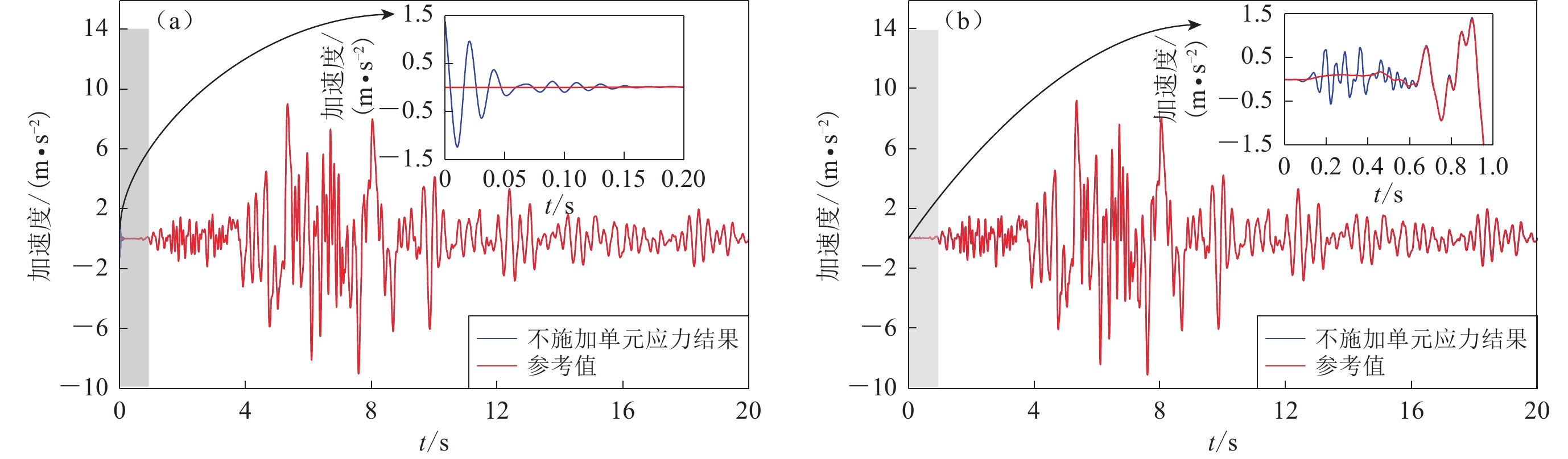
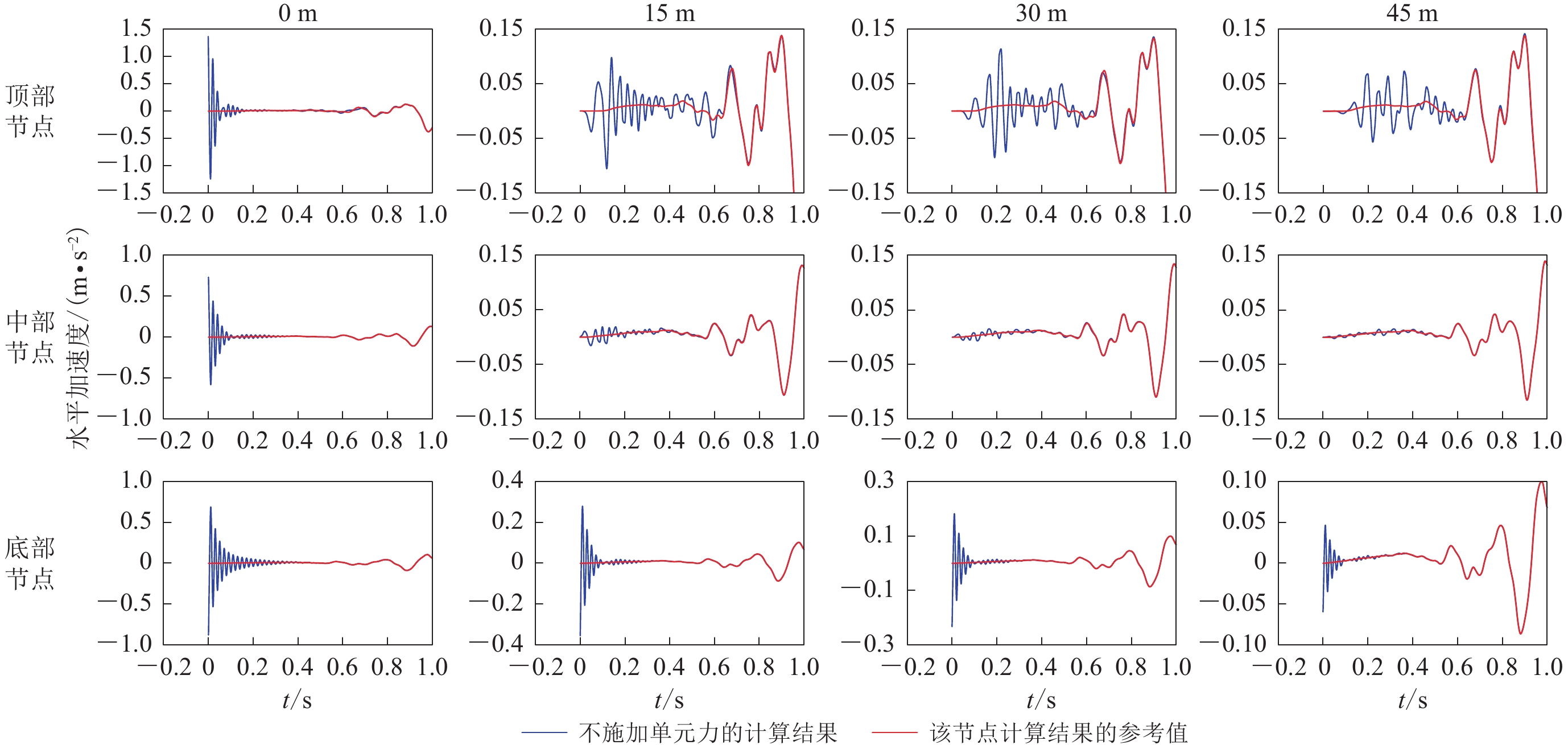
为了分析模型在不合理静动力边界转换方法下振荡程度以及更好地给出参考解法的使用方法,在本节的自由场模型中设置12个水平加速度监测点,如图2中红色点所示,监测点从模型左边界开始,相邻监测点之间间隔15 m。图10比较了模型左边界及中部的顶部节点的水平加速度时程与对应参考模型的参考值。分析可知,对于模型边界顶部节点和模型顶部中点,不合理的静动力边界转换对初始阶段的水平加速度有一定影响,而后续加速度时程曲线与参考解基本一致。图11给出了12个不同监测点在第一秒内地震荷载下的水平加速度动力响应。分析可知,对于处在同一深度的节点,越靠近左侧边界,不合理静动力转换引起的振荡强度越大,模型中间位置节点的振荡最小;此外,所有边界上的监测点(N1—N6)振荡均比其它位置监测点强烈,侧边界顶部节点N1的振荡强度最大。这可能是自由场放大效应和不平衡力共同作用的结果。因此,在使用参考解方法时,建议选取侧边界底部、顶部节点和模型中部顶部和底部的节点的加速度动力响应来比较验证,确认静动力边界转换合理性及黏弹性边界的正确施加和地震动的正确输入。以上结果表明,不施加单元应力的静动力边界转换方法,在弹性条件下,会对动力计算结果加速度的初始阶段产生一定的影响(振荡),而后阶段与参考解基本一致,边界顶部节点的动力响应影响较中间节点更大。
![]() 图 10 模型左边界(a)及中部(b)的顶部节点水平加速度时程Figure 10. Acceleration time history of nodes at the top of the left boundary (a) and the vertical middle model (b)
图 10 模型左边界(a)及中部(b)的顶部节点水平加速度时程Figure 10. Acceleration time history of nodes at the top of the left boundary (a) and the vertical middle model (b)![]() 图 11 不合理静动力边界转换下模型不同位置节点水平加速度时程曲线Figure 11. Horizontal acceleration time history of different nodes with unreasonable static-dynamic boundary switch method
图 11 不合理静动力边界转换下模型不同位置节点水平加速度时程曲线Figure 11. Horizontal acceleration time history of different nodes with unreasonable static-dynamic boundary switch method4.2 振荡产生的原因和机理
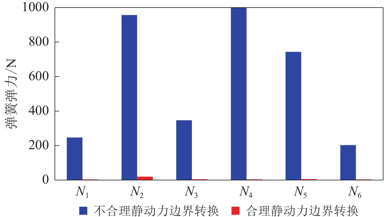
黏弹性边界是由模型边界上的并联的弹簧阻尼系统构成,是一种应力型边界。由式(2)可知,在地震输入时,需要输入的等效节点力必须要能够克服弹簧和阻尼器产生的附加应力以及自由场地震动在边界上产生的应力,使得边界与自由场运动一致,才能保证边界上的位移和应力边界条件的连续。由4.1节可知,不合理的静动力边界转换后加速度时程振荡在模型侧面和底面最显著,因此为探究其振荡原因,输出进行合理静动力边界转换和不合理转换两种情况下,多土层自由场模型黏弹性边界节点(N1—N6)上弹簧单元在进行静动力边界转换后动力分析步前的弹力绝对值如图12所示。分析可知,不合理静动力边界转换模型边界节点弹簧在动力分析步前已经有很大的弹力,表明静动力边界转换后有力作用在黏弹性边界弹簧单元上,此力称为不平衡力。模型整个体系的地应力平衡是重力及其引起的单元内力和边界反力平衡的结果,因此去掉边界后除了施加边界节点反力外,不施加重力或模型单元内力,必然会使弹簧变形并产生附加应力,意味着动力分析步中地震动(等效节点力)的施加将出现误差。所以在进行土-地下结构静动力耦合动力计算分析时,必须保证静力边界转换成动力边界过程中,整个计算模型处于静力平衡状态,黏弹性边界上不能受到不平衡力的作用,否则会在动力分析步初始时刻引起动力效应,具体表现为模型在未受到地震动力荷载作用前,模型节点动力响应已经出现了较大振荡,最终导致地震动力计算结果不合理。
![]() 图 12 多土层自由场模型黏弹性边界节点弹簧弹力受力情况Figure 12. The magnitude of elastic fore for spring elements located at the viscous-spring boundary
图 12 多土层自由场模型黏弹性边界节点弹簧弹力受力情况Figure 12. The magnitude of elastic fore for spring elements located at the viscous-spring boundary5. 结 论
本文根据弹性叠加原理,提出了一种验证静动力边界转换合理性的方法即参考解法,利用有限元程序ABAQUS,并结合自编等效节点力的计算程序以及黏弹性边界的自动施加程序VBEA2.0,建立了二维成层自由场静动力耦合模型和土-地下结构静动力耦合模型,对比分析了参考解法的适用性;在此基础上,针对黏弹性边界条件下传统静动力边界转换过程出现的振荡反应现象进行了相关研究,探讨了造成振荡的原因和机理。主要结论如下:
1) 合理考虑其静动力耦合效应需要遵循以下程序:首先进行地应力平衡静力计算;然后进行静动力边界转换;最后进行动力计算。在静动力边界转换过程中,除施加边界节点反力来替代静力边界条件外,还需施加所有单元的应力场以及重力场。
2) 根据二维成层自由场静动力耦合模型和土-地下结构静动力耦合模型的计算分析结果,以不考虑静动力耦合作用的模型计算结果作为动力反应分析的参考解来判断静动力边界转换的合理性方法(参考解法),能够较好地验证静动力边界转换的合理性,并且能直观地反映出动力计算初期是否有波动以及波动对后阶段动力计算的影响程度。该方法可在土-地下结构的静动力耦合动力分析中为静动力边界转换的合理性检验提供一种有效工具。
3) 静动力耦合计算模型静力不平衡是导致静动力边界转换出现振荡的物理机制;边界反力、重力、单元应力的施加合理与否是影响静动力边界的不合理转换的主要因素。
-
![]()
图 1 静动力边界转换方法示意图
(a) 地应力平衡;(b) 静动力边界转化;(c) 施加地震荷载
Figure 1. Schematic diagram of static-dynamic boundary switch
(a) In-situ stress balance;(b) Switching between static and dynamic boundary;(c) Application of earthquake loading
![]()
图 3 日本神户地震南北分量加速度时程
Figure 3. Acceleration time history of the north and south components of the Kobe earthquake
![]()
图 4 自由场地震反应计算结果
(a) 100 m×50 m模型峰值加速度;(b) 100 m×50 m模型最大相对位移;(c) 200 m×100 m模型峰值加速度;(d) 200 m×100 m模型最大相对位移;(e) 随深度变化的加速度、位移时程误差
Figure 4. Seismic dynamic response of free field
(a) Maximum acceleration for 100 m×50 m model;(b) Maximum relative displacement for 100 m×50 m model;(c) Maximum acceleration for 200 m×100 m model;(d) Maximum relative displacement for 200 m×100 m model;(e) Acceleration and displacement time-history errors with varying depths
![]()
图 7 带地下结构的成层场地地震动力反应计算结果
(a) 场地土PGA;(b) 场地土最大相对位移;(c) 车站中柱最大相对位移;(d) 车站结构重要部位最大主应力
Figure 7. Earthquake dynamic response of underground structure in the layered site
(a) Maximum acceleration of the site;(b) Maximum relative displacement of the site;(c) Maximum relative displacement of the central column;(d) Maximum principal stress at points in the station
![]()
图 8 带地下结构的成层场地左边界及中部节点水平向的加速度时程(左)和位移时程(右)
(a) 左边界顶部节点;(b) 地表中部节点;(c) 左边界底部节点;(d) 底边界中部节点
Figure 8. Horizontal acceleration (left) and displacement (right) time history of nodes at the left boundary and the vertical middle of underground structure in the layered site
(a) Node at the top of the left boundary;(b) Node at the centre of the surface;(c) Node at the bottom of the left boundary;(d) Node at the centre of the base
![]()
图 9 带地下结构的成层场地地震动力反应时程结果误差
Figure 9. The error of the earthquake dynamic response of sub-structure in the layered site
![]()
图 10 模型左边界(a)及中部(b)的顶部节点水平加速度时程
Figure 10. Acceleration time history of nodes at the top of the left boundary (a) and the vertical middle model (b)
![]()
图 11 不合理静动力边界转换下模型不同位置节点水平加速度时程曲线
Figure 11. Horizontal acceleration time history of different nodes with unreasonable static-dynamic boundary switch method
![]()
图 12 多土层自由场模型黏弹性边界节点弹簧弹力受力情况
Figure 12. The magnitude of elastic fore for spring elements located at the viscous-spring boundary
表 1 大开地铁车站数值模型场地条件参数
Table 1 Mechanical parameters of the soil layers for the Dakai metro station
土质 模型各层厚度/m 密度/(kg·m−3) 较软地层模型vS
/(m·s−1)真实地层模型vS
/(m·s−1)较硬地层模型vS
/(m·s−1)泊松比 人工填土 1 1 900 80 140 290 0.333 全新世砂土 4 1 900 80 140 290 0.320 全新世砂土 3 1 900 110 170 320 0.320 更新世黏土 3 1 900 130 190 340 0.400 更新世黏土 6 1 900 180 240 390 0.300 更新世砂土 5 2 000 270 330 480 0.260 基岩 20 2 000 1 000 1 000 1 000 0.260  下载: 导出CSV
-
曹炳政,罗奇峰,马硕,刘晶波. 2002. 神户大开地铁车站的地震反应分析[J]. 地震工程与工程振动,22(4):102–107. Cao B Z,Luo Q F,Ma S,Liu J B. 2002. Seismic response analysis of Dakai subway station in Hyogoken-Nanbu earthquake[J]. Earthquake Engineering and Engineering Vibration,22(4):102–107 (in Chinese).
陈国兴. 2007. 岩土地震工程学[M]. 北京: 科学出版社: 557−558. Chen G X. 2007. Geotechnical Earthquake Engineering[M]. Beijing: Science Press: 557−558 (in Chinese).
杜修力,涂劲,陈厚群. 2000. 有缝拱坝-地基系统非线性地震波动反应分析方法[J]. 地震工程与工程振动,20(1):11–20. Du X L,Tu J,Chen H Q. 2000. Nonlinear seismic response analysis of arch dam-foundation systems with cracked surfaces[J]. Earthquake Engineering and Engineering Vibration,20(1):11–20 (in Chinese).
付培帅. 2015. 预应力大跨地铁站震害机理与结构优选研究[D]. 大连: 大连理工大学: 32–37. Fu P S. 2015. Study on Earthquake Damage Mechanism and Structure Selection of Prestressed Large-Span Subway Station[D]. Dalian: Dalian University of Technology: 32–37 (in Chinese).
高峰,赵冯兵. 2011. 地下结构静-动力分析中的人工边界转换方法研究[J]. 振动与冲击,30(11):165–170. Gao F,Zhao F B. 2011. Study on transformation method for artificial boundaries in static-dynamic analysis of underground structure[J]. Journal of Vibration and Shock,30(11):165–170 (in Chinese).
郭亚然,石文倩,李双飞,蒋录珍. 2018. 静、动力分析中的一种初始地应力场平衡方法[J]. 河北工业科技,35(3):191–196. Guo Y R,Shi W Q,Li S F,Jiang L Z. 2018. A method of initial geo-stress equilibrium in static-dynamic analysis[J]. Hebei Journal of Industrial Science &Technology,35(3):191–196 (in Chinese).
廖维张,杜修力,赵密,李立云. 2006. 开放系统非线性动力反应分析的一种算法[J]. 北京工业大学学报,32(2):115–119. Liao W Z,Du X L,Zhao M,Li L Y. 2006. An algorithm of the non-linear dynamic analysis of open system[J]. Journal of Beijing University of Technology,32(2):115–119 (in Chinese).
廖振鹏,黄孔亮,杨柏坡,袁一凡. 1984. 暂态波透射边界[J]. 中国科学(A辑),(6):556–564. Liao Z P,Huang K L,Yang B P,Yuan Y F. 1984. Transient wave transmission boundary[J]. Science in China:Series A,14(6):556–564 (in Chinese).
廖振鹏,刘晶波. 1986. 离散网格中的弹性波动(Ⅰ)[J]. 地震工程与工程振动,6(2):1–16. Liao Z P,Liu J B. 1986. Elastic wave motion in discrete grids[J]. Earthquake Engineering and Engineering Vibration,6(2):1–16 (in Chinese).
刘晶波,李彬. 2005. 三维黏弹性静-动力统一人工边界[J]. 中国科学:E辑 工程科学 材料科学,35(9):966–980. Liu J B,Li B. 2005. A unified viscous-spring artificial boundary for 3-D static and dynamic applications[J]. Science in China:Series E Engineering &Materials Science,48(5):570–584.
刘晶波, 杜义欣, 闫秋实. 2007. 粘弹性人工边界及地震动输入在通用有限元软件中的实现[C]//第三届全国防震减灾工程学术研讨会. 南京: 中国土木工程学会: 37–42. Liu J B, Du Y X, Yan Q S. 2007. Viscous-elastic artificial boundary and earthquake dynamic input in common finite element software[C]//National Seismic on Earthquake Prevention and Disaster Reduction Engineering. Nanjing: China Civil Engineering Society: 37–42 (in Chinese).
马笙杰,迟明杰,陈红娟,陈苏. 2020. 黏弹性人工边界在ABAQUS中的实现及地震动输入方法的比较研究[J]. 岩石力学与工程学报,39(7):1445–1457. Ma S J,Chi M J,Chen H J,Chen S. 2020. Implementation of viscous-spring boundary in ABAQUS and comparative study on seismic motion input methods[J]. Chinese Journal of Rock Mechanics and Engineering,39(7):1445–1457 (in Chinese).
马笙杰. 2021. 凸起地形与上覆土层对强地震动特性的影响研究[D]. 北京: 中国地震局地球物理研究所: 22–30. Ma S J. 2021. Research on the Influence of Convex Topography and Overlying Soil on the Characteristics of Strong Ground Motion[D]. Beijing: Institute of Geophysics, China Earthquake Administration: 22–30 (in Chinese).
王苏,路德春,杜修力. 2012. 地下结构地震破坏静-动力耦合模拟研究[J]. 岩土力学,33(11):3483–3488. Wang S,Lu D C,Du X L. 2012. Research on underground structure seismic damage using static-dynamic coupling simulation method[J]. Rock and Soil Mechanics,33(11):3483–3488 (in Chinese).
Deeks A J,Randolph M F. 1994. Axisymmetric time-domain transmitting boundaries[J]. Journal of Engineering Mechanics,120(1):25–42. doi: 10.1061/(ASCE)0733-9399(1994)120:1(25)
Su W,Qiu Y X,Xu Y J,Wang J T. 2021. A scheme for switching boundary condition types in the integral static-dynamic analysis of soil-structures in Abaqus[J]. Soil Dynamics and Earthquake Engineering,141:106458. doi: 10.1016/j.soildyn.2020.106458
Ungless R F. 1973. An Infinite Finite Element[D]. Vancouver: University of British Columbia: 50.
-
期刊类型引用(1)
1. 薛景宏,陆大伟,李东瑞,程安顿,韩通. 地震波斜入射下埋地腐蚀管道地震响应分析. 河北工程大学学报(自然科学版). 2024(04): 18-27+35 .  百度学术
百度学术
其他类型引用(1)

计量
- 文章访问数: 619
- HTML全文浏览量: 80
- PDF下载量: 162
- 被引次数: 2
